Final Exam — Spring 2025: Worked Solutions

Exam Information

Course: STAT 350 — Introduction to Statistics

Semester: Spring 2025

Total Points: 150 + 15 (Extra Credit) = 165

Time Allowed: 120 minutes

Coverage: Cumulative (Chapters 1–13); primary emphasis on Chapters 12–13, with Chapters 1–7 weighted more heavily than Chapters 8–11 among the earlier material

Problem	Total Possible	Topic
Problem 1 (True/False, 2 pts each)	12	Covariance/Correlation, CLT/Binomial, Bayes’ Theorem, ANOVA F-test, Least Squares, Extrapolation
Problem 2 (Multiple Choice, 3 pts each)	18	Probability Inequalities, Random Variable Properties, Two-Sample Inference, SLR Units, Residual Patterns, ANOVA MSE Bias
Problem 3 (Matching)	21	Confidence Intervals/Bounds, Sampling Bias, Paired Design, Interval Width, Interpretation Errors
Problem 4	32	Exponential Distribution, Laplace Distribution, CLT/Sampling Distribution
Problem 5	40	Simple Linear Regression
Problem 6	42	One-Way ANOVA, Tukey HSD
Total	150 (+ 15 Extra Credit)

—

Problem 1 — True/False (12 points, 2 pts each)

Question 1.1 (2 pts)

Suppose \(X\) and \(Y\) are two random variables with a large covariance \(\text{COV}(X, Y) = 100{,}000\), and the individual standard deviations \(\sigma_X\) and \(\sigma_Y\) are unknown but finite. From this information, we can conclude that \(X\) and \(Y\) are strongly correlated.

Solution

Answer: FALSE

The correlation coefficient is defined as:

\[\rho = \frac{\text{COV}(X, Y)}{\sigma_X \sigma_Y}\]

A large covariance does not imply strong correlation because the covariance is not scale-free. If \(\sigma_X\) and \(\sigma_Y\) are very large, \(\rho\) could be close to zero even with \(\text{COV}(X, Y) = 100{,}000\). Since \(\sigma_X\) and \(\sigma_Y\) are unknown, we cannot determine the value of \(\rho\) and therefore cannot conclude strong correlation.

Question 1.2 (2 pts)

A Reddit user claims that when one encounters a Pokémon in the wild, there is a 2% chance that it is a legendary Pokémon. Assume that each encounter is independent, each has the same 2% chance, and each wild Pokémon encountered is either legendary or not legendary. Assuming the claim is true: the number of legendary Pokémon encountered is approximately normal if a sufficiently large number of wild Pokémon are observed.

Solution

Answer: TRUE

Let \(X\) = number of legendary Pokémon encountered in \(n\) encounters. Then \(X \sim \text{Binomial}(n, p = 0.02)\). Since each encounter is an independent Bernoulli trial, the CLT applies to the sum \(X\). For sufficiently large \(n\) such that \(np \geq 10\) and \(n(1-p) \geq 10\) (i.e., \(n \geq 500\)), the sampling distribution of \(X\) is approximately normal.

Question 1.3 (2 pts)

Bayes’ Theorem is often used for revising probabilities based on new evidence. Bayes’ Theorem applies when the events of interest, \(A_1, A_2, \ldots, A_k\), are mutually exclusive (disjoint), and the evidence event \(B\) has positive probability.

Solution

Answer: TRUE

Bayes’ Theorem states:

\[P(A_i \mid B) = \frac{P(B \mid A_i)\,P(A_i)}{\sum_{j=1}^{k} P(B \mid A_j)\,P(A_j)}\]

The denominator is the Law of Total Probability, which requires the \(A_j\) to be mutually exclusive and exhaustive, and \(P(B) > 0\). The statement is TRUE, noting that the \(A_i\) must also be exhaustive (collectively covering the entire sample space), though the question focuses on the mutual exclusivity and positive-probability conditions.

Question 1.4 (2 pts)

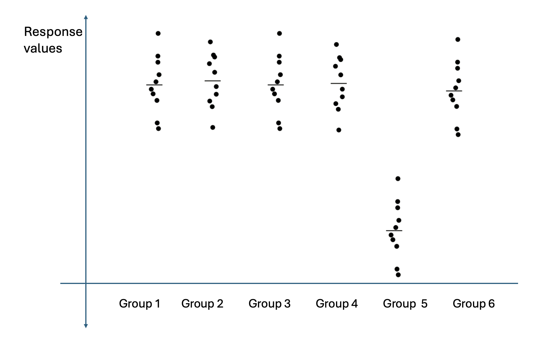
The plot below shows the response values of an experiment organized by different treatment groups. According to the plot, an ANOVA F-test for this dataset will most likely result in a failure to reject \(H_0\) because most groups are shaped very similarly.

Solution

Answer: FALSE

While most groups (1–5) do appear to have similar shapes and centers, Group 6 has a noticeably lower mean response, well separated from the others. The ANOVA F-test detects differences in group means — it does not require all groups to differ. The visual separation of Group 6 indicates that at least one pair of means differs, so the F-test will most likely reject \(H_0\), not fail to reject it.

Question 1.5 (2 pts)

Let \(\hat{\beta}_1\) and \(\hat{\beta}_0\) be the slope and intercept of the regression line computed from a dataset \((x_1, y_1), (x_2, y_2), \ldots, (x_n, y_n)\). Suppose a function \(l\) is defined as:

\[l(a, b) = \sum_{i=1}^{n} \bigl(y_i - (a + b x_i)\bigr)^2\]

Then \(l\) attains the smallest value possible by plugging in \(\hat{\beta}_0\) for \(a\) and \(\hat{\beta}_1\) for \(b\).

Solution

Answer: TRUE

The function \(l(a, b)\) is precisely the sum of squared residuals (SSE) as a function of the intercept \(a\) and slope \(b\). The least squares estimators \(\hat{\beta}_0\) and \(\hat{\beta}_1\) are defined as the values of \((a, b)\) that minimize \(l(a, b)\) over all possible choices of \(a\) and \(b\). Therefore, \(l(\hat{\beta}_0, \hat{\beta}_1) \leq l(a, b)\) for all \((a, b)\), and the statement is TRUE.

Question 1.6 (2 pts)

Interpolation and extrapolation are terms used for making predictions with a regression model. Extrapolation typically yields safer, more reliable predictions than interpolation.

Solution

Answer: FALSE

Interpolation — predicting within the observed range of \(x\) values — is generally safer because the linear model has been empirically validated over that range. Extrapolation — predicting outside the observed range — is unreliable because the linear relationship may not hold beyond the data, and small errors in the estimated slope are amplified over large \(x\)-distances. Extrapolation is therefore riskier, not safer.

—

Problem 2 — Multiple Choice (18 points, 3 pts each)

Question 2.1 (3 pts)

Suppose \(A\), \(B\), \(C\), and \(D\) are non-empty events in the same sample space where \(P(C) > P(A \cup B) > P(D) > 0.7\). Which of the following statements is TRUE?

• 1. \(D\) must be a subset of \(C\).

• 2. \(P(A' \cap B') < P(C') < 0.3\) holds.

• 3. The two events \(C\) and \(D\) can be mutually exclusive.

• 4. If \(A \cap C = \emptyset\), then \(B \cap C\) must be a non-empty set.

• 5. The two events \(A\) and \(B\) are independent.

Solution

Answer: (D)

Since \(P(C) > P(A \cup B) > 0.7\), we have \(P(C) + P(A \cup B) > 1.4 > 1\). By inclusion-exclusion:

\[P\!\bigl(C \cap (A \cup B)\bigr) \geq P(C) + P(A \cup B) - 1 > 0.4 > 0\]

So \(C\) and \(A \cup B\) must overlap. Since \(C \cap (A \cup B) = (C \cap A) \cup (C \cap B)\), if \(A \cap C = \emptyset\) then \(C \cap (A \cup B) = C \cap B = B \cap C\). Therefore \(P(B \cap C) > 0\), which means \(B \cap C\) must be a non-empty set. (D) is TRUE.

• (A) FALSE. High probability of \(D\) does not imply \(D \subseteq C\); subset relationships depend on set containment, not just probability values.

• (B) FALSE. Since \(P(C) > P(A \cup B)\), we have \(P(C') = 1 - P(C) < 1 - P(A \cup B) = P(A' \cap B')\). So the correct ordering is \(P(C') < P(A' \cap B') < 0.3\) — the inequality in option (B) is reversed.

• (C) FALSE. If \(C\) and \(D\) were mutually exclusive, \(P(C \cup D) = P(C) + P(D) > 0.7 + 0.7 = 1.4 > 1\), which is impossible.

• (E) FALSE. The given probability inequalities place no constraint on whether \(A\) and \(B\) are independent.

Note on solution key ⚠️

The solution key marks (B) as the answer, but option (B) states \(P(A' \cap B') < P(C') < 0.3\). Because \(P(C) > P(A \cup B)\), we in fact have \(P(C') < P(A' \cap B')\) — the inequality is reversed, making (B) false. Option (D) is the correct answer, as shown above.

Question 2.2 (3 pts)

Which statement regarding the properties of common random variables is FALSE?

• 1. A Poisson random variable counts the number of events occurring in a fixed interval of time, area, or space.

• 2. A Uniform random variable assigns equal probability density across its entire support.

• 3. A Binomial random variable counts the number of independent trials required to achieve a specified number of successes.

• 4. An Exponential random variable measures the waiting time between consecutive independent events.

• 5. None of the statements listed above are false.

Solution

Answer: (C)

• (A) TRUE. Poisson counts events in a fixed interval.

• (B) TRUE. Uniform assigns constant density \(1/(b-a)\) over \([a, b]\).

• (C) FALSE. A Binomial random variable counts the number of successes in a fixed number \(n\) of independent trials — not the number of trials needed. The description in (C) (counting trials to a specified number of successes) describes the Negative Binomial distribution, which is not covered in this course.

• (D) TRUE. The Exponential distribution models waiting times between consecutive events in a Poisson process.

Question 2.3 (3 pts)

In an Amish community, an accountant wants to determine if the daily profit from selling groceries has increased in 2024 compared to 2023. However, due to a recent flood, the accountant was only able to obtain daily profit data for 55 days in 2023 and 82 days in 2024. The calculated test statistic follows the \(t\)-distribution with \(\text{df} \approx 117.25\). Historically the distribution of daily profit prior to 2023 exhibited slight positive skewness, and current samples appear consistent with historical patterns. Which of the following statements in the accountant’s report is FALSE?

• 1. Daily profit reports were mixed in a random order, and only a few reports at the top of the pile were readable after the flood. Thus, the SRS assumption is naively satisfied.

• 2. Since the daily profit is measured for the same Amish community in both years, a two-sample matched-pairs t-test should be used for analysis.

• 3. The combined sample size is sufficiently large for the t-test to be robust against slight positive skewness.

• 4. A \(Z\)-table is used when calculating the \(p\)-value due to limited access to electricity. The use of a \(Z\)-table is a reasonable approximation because the \(t\)-distribution becomes approximately Normal when df is sufficiently large.

Solution

Answer: (B)

• (A) TRUE (plausible). If reports were randomly mixed and the top few happened to be readable, this is a rough justification for treating the available records as an SRS. The statement is described as “naively satisfied” — indicating a weak but defensible assumption.

• (B) FALSE. A matched-pairs design requires one-to-one pairing of observations (e.g., the same day in both years, or the same individual measured twice). Here the data are separate samples of 55 days and 82 days — there is no natural pairing because the sample sizes differ and the days are not matched. A two-sample independent \(t\)-test (Welch’s, since \(\text{df} \approx 117.25\) suggests unequal variances) is appropriate.

• (C) TRUE. With combined \(n = 55 + 82 = 137\), the CLT provides adequate robustness against slight skewness.

• (D) TRUE. With \(\text{df} \approx 117\), the \(t\)-distribution is nearly indistinguishable from the standard normal, making the \(Z\)-table a reasonable approximation.

Question 2.4 (3 pts)

In a simple linear regression, the predictor variable is recorded in pounds (lbs). What restriction, if any, does this put on the units of the response variable?

• 1. It must be measured in some other unit of mass or weight.

• 2. It cannot be expressed in pounds or any other weight units.

• 3. It may be measured in whatever units are appropriate for the outcome.

• 4. It must be measured in pounds exactly, matching the predictor units.

• 5. Each of the statements given above is simultaneously valid and applicable.

Solution

Answer: (C)

In simple linear regression \(\hat{Y} = b_0 + b_1 x\), the slope \(b_1\) has units of (response units)/(predictor units), and the intercept \(b_0\) has units of the response. There is no restriction on the units of \(Y\) imposed by the units of \(x\). The response variable may be measured in any units appropriate for the application — they need not match, relate to, or differ from the predictor’s units.

Question 2.5 (3 pts)

If the error variance is constant across all values of the predictor (homoscedasticity), what overall pattern should appear in a plot of residuals versus the predictor?

• 1. The residuals spread out progressively, forming a fan shape.

• 2. The residual spread narrows progressively, forming a funnel shape.

• 3. Residual spread first widens and then narrows across the range.

• 4. Residual spread stays about the same, forming a uniform band.

• 5. Residuals align along a single slanted line rising or falling.

Solution

Answer: (D)

Under homoscedasticity the variance of \(\varepsilon_i\) is constant at \(\sigma^2\) for all values of \(x\). In the residual plot this manifests as a roughly uniform horizontal band of scatter — no systematic widening (fan), narrowing (funnel), or other patterns related to the predictor value. Options (A)–(C) describe heteroscedasticity; (E) describes a non-zero slope remaining in the residuals, which indicates a violation of linearity.

Question 2.6 (3 pts)

A researcher performs ANOVA to analyze a dataset, and they mistakenly used the entire sample size \(n\) instead of \(n_i\) when calculating group variances \(s_i^2\). Assuming the formula below was used for calculating the MSE value, which of the following statements is TRUE?

\[\text{MSE} = \frac{\sum_{i=1}^{k}(n_i - 1)s_i^2}{n - k}\]

• 1. The MSE value is overestimated, so it increases the chance of rejecting \(H_0\).

• 2. The MSE value is overestimated, so it decreases the chance of rejecting \(H_0\).

• 3. The MSE value is overestimated, but the ANOVA results remain the same.

• 4. The MSE value is underestimated, so it increases the chance of rejecting \(H_0\).

• 5. The MSE value is underestimated, so it decreases the chance of rejecting \(H_0\).

• 6. The MSE value is underestimated, but the ANOVA results remain the same.

Solution

Answer: (D)

If the researcher uses \(n\) (total sample size) as the denominator instead of \(n_i\) when computing each group’s sample variance, the resulting variance estimate is:

\[s_{i,\text{wrong}}^2 = \frac{\sum_{j=1}^{n_i}(x_{ij} - \bar{x}_i)^2}{n - 1}\]

Since \(n > n_i\), the denominator \(n - 1\) is larger than the correct \(n_i - 1\), so \(s_{i,\text{wrong}}^2 < s_i^2\) for each group. The MSE numerator \(\sum_{i=1}^{k}(n_i-1)s_i^2\) uses these deflated variance estimates, so the overall MSE is underestimated. A smaller MSE inflates the F-statistic \(F_{\text{TS}} = \text{MSA}/\text{MSE}\), which increases the chance of rejecting \(H_0\). Therefore (D) is correct.

—

Problem 3 Setup

A biological research firm hired seven new intern statisticians. As part of their training program, the firm requires each intern to run a mock experiment and submit a report answering a unique statistical question. Being new to the position, the interns made various mistakes during this procedure.

The consequence choices are:

Letter	Consequence
A	The margin of error will be larger than necessary.
B	The margin of error will be smaller than necessary.
C	The sample will be a biased representation of the population.
D	The result will be impacted by extraneous variation.
E	An inaccurate message about the result will be conveyed to the non-statisticians in their team.
F	This does not lead to any serious consequences.

Problem 3 — Matching (21 points, 3 pts each)

Question 3 — All seven interns (21 pts)

Match each intern’s mistake to its most serious consequence (A–F).

Arthur created a two-sided confidence interval, while a one-sided lower confidence bound was necessary.

Bill asked all his extended family members to participate in his experiment in order to expedite data collection.

Charlie used a two-sample independent approach, while it was correct to use the matched-pairs approach.

Ron was unaware that the population SD was known, so he instead used the sample SD and the \(t\)-procedure to create a lower confidence bound.

Molly correctly obtained a lower confidence bound of −0.73 with 95% confidence. She reported that “the true parameter is above −0.73 with probability 0.95.”

Fred rejected the null hypothesis for an ANOVA F-test and proceeded to construct confidence intervals for pairwise differences of means using the Bonferroni method. Given the family-wise Type I error \(\alpha\), he used the critical value \(t_{\alpha/2,\,\text{df}}\) for each interval.

Ginny conducted the F-test for linear regression and failed to reject the null hypothesis. She reported that the explanatory variable and the response variable “can be seen as independent of each other.”

Solution

Matching Answers

Intern	Answer	Explanation
Arthur	A	A two-sided confidence interval has a critical value \(z_{\alpha/2}\) (or \(t_{\alpha/2}\)), while a one-sided lower confidence bound uses the smaller critical value \(z_\alpha\). The CI extends in both directions, so it is wider — the margin of error is larger than necessary for the one-sided inference goal.
Bill	C	Recruiting only family members is a convenience sample (voluntary/network sampling). Family members likely share characteristics — lifestyle, economics, genetics — that are not representative of the broader population. The sample will be a biased representation of the population.
Charlie	D	When a matched-pairs design is appropriate (e.g., before/after measurements on the same subject or paired subjects), using a two-sample independent approach fails to remove the within-pair correlation. The extraneous between-subject variation that the pairing was designed to eliminate remains in the error, inflating the variance estimate. The result will be impacted by extraneous variation.
Ron	A	When \(\sigma\) is known, the \(z\)-procedure should be used; critical values from \(z\) are smaller than the corresponding \(t\) critical values (since the \(t\)-distribution has heavier tails). Using \(t\) when \(z\) is appropriate produces a larger margin of error than necessary.
Molly	E	The lower confidence bound of −0.73 is a fixed number computed from the data; the true parameter is also a fixed (though unknown) constant — it is not a random variable. Saying “the true parameter is above −0.73 with probability 0.95” assigns a probability to a fixed event, which is a frequentist error. The correct statement is “We are 95% confident that the true parameter is greater than −0.73.” This conveys an inaccurate message about the nature of the result.
Fred	B	The Bonferroni correction for \(C = \binom{k}{2}\) pairwise comparisons uses critical value \(t_{\alpha/(2C),\,\text{df}}\), not \(t_{\alpha/2,\,\text{df}}\). Since \(\alpha/2 > \alpha/(2C)\), Fred’s critical value is smaller than it should be, producing confidence intervals that are narrower than necessary — the margin of error is smaller than necessary, and the family-wise Type I error is inflated.
Ginny	E	Failing to reject \(H_0\colon \beta_1 = 0\) means there is insufficient evidence of a linear association. It does not mean the variables are statistically independent — a nonlinear relationship could still exist. Reporting “the variables can be seen as independent” overstates the conclusion and conveys an inaccurate message to the team.

—

Problem 4 Setup

At a high-frequency trading venue, the waiting time (in milliseconds) until the next buy order arrives follows \(T_{\text{Buy}} \sim \text{Exp}(\lambda_{\text{Buy}})\), and the waiting time until the next sell order arrives independently follows \(T_{\text{Sell}} \sim \text{Exp}(\lambda_{\text{Sell}})\).

Define the signed arrival-time difference:

\[R = T_{\text{Buy}} - T_{\text{Sell}}\]

Problem 4 — Exponential Distribution, Laplace, and CLT (32 points)

Question 4a (4 pts)

Assume \(\lambda_{\text{Buy}} = 3\ \text{ms}^{-1}\) and \(\lambda_{\text{Sell}} = 1\ \text{ms}^{-1}\). Determine \(E[R]\) and \(\text{Var}(R)\).

Solution

For \(T \sim \text{Exp}(\lambda)\): \(E[T] = 1/\lambda\) and \(\text{Var}(T) = 1/\lambda^2\). Since \(T_{\text{Buy}}\) and \(T_{\text{Sell}}\) are independent:

\[E[R] = E[T_{\text{Buy}}] - E[T_{\text{Sell}}] = \frac{1}{3} - \frac{1}{1} = -\frac{2}{3} \approx \boxed{-0.6667}\]

\[\text{Var}(R) = \text{Var}(T_{\text{Buy}}) + \text{Var}(T_{\text{Sell}}) = \frac{1}{3^2} + \frac{1}{1^2} = \frac{1}{9} + 1 = \frac{10}{9} \approx \boxed{1.1111}\]

(The variance of \(-T_{\text{Sell}}\) equals \(\text{Var}(T_{\text{Sell}})\) since variance is unaffected by sign.)

Question 4b (12 pts)

Under these assumptions, \(R\) follows a Laplace (double-exponential) distribution with parameters \(\mu = E[R]\) and \(b = 1/\lambda_{\text{Buy}} + 1/\lambda_{\text{Sell}}\). The pdf is:

\[\begin{split}f_R(x) = \begin{cases} \dfrac{1}{2b}\,e^{(x-\mu)/b} & x < \mu \\[6pt] \dfrac{1}{2b}\,e^{-(x-\mu)/b} & x \geq \mu \end{cases}\end{split}\]

Write down the parameters \(\mu\) and \(b\), and compute \(P(-1 \leq R \leq 1)\).

Solution

Parameters:

\[\mu = -\frac{2}{3}, \qquad b = \frac{1}{3} + \frac{1}{1} = \frac{4}{3} \approx 1.3333\]

So \(\frac{1}{2b} = \frac{3}{8}\) and the exponent coefficient is \(\frac{1}{b} = \frac{3}{4}\).

Computing \(P(-1 \leq R \leq 1)\): split the integral at \(\mu = -2/3\).

\[P(-1 \leq R \leq 1) = \frac{3}{8}\left[\int_{-1}^{-2/3} e^{\frac{3}{4}(x+\frac{2}{3})}\,dx + \int_{-2/3}^{1} e^{-\frac{3}{4}(x+\frac{2}{3})}\,dx\right]\]

Substitute \(u = x + 2/3\), so \(du = dx\):

\[= \frac{3}{8}\left[\int_{-1/3}^{0} e^{\frac{3}{4}u}\,du + \int_{0}^{5/3} e^{-\frac{3}{4}u}\,du\right]\]

Evaluating each integral:

\[= \frac{3}{8}\left[\frac{4}{3}\!\left(1 - e^{-1/4}\right) + \frac{4}{3}\!\left(1 - e^{-5/4}\right)\right]\]

\[= \frac{1}{2}\!\left(1 - e^{-1/4}\right) + \frac{1}{2}\!\left(1 - e^{-5/4}\right) = 1 - \frac{1}{2}\!\left(e^{-1/4} + e^{-5/4}\right)\]

\[= 1 - \frac{1}{2}(0.7788 + 0.2865) = 1 - 0.5327 = \boxed{0.4673}\]

Question 4c (6 pts)

Suppose we record the next 55 independent observations \(R_1, R_2, \ldots, R_{55}\), each following the same Laplace distribution. Define:

\[\bar{R} = \frac{1}{55}\sum_{i=1}^{55} R_i\]

Determine the exact mean \(E[\bar{R}]\) and variance \(\text{Var}(\bar{R})\).

Solution

By the properties of sample means of i.i.d. random variables:

\[E[\bar{R}] = E[R] = \boxed{-\frac{2}{3} \approx -0.6667}\]

\[\text{Var}(\bar{R}) = \frac{\text{Var}(R)}{n} = \frac{10/9}{55} = \frac{10}{495} = \frac{2}{99} \approx \boxed{0.0202}\]

Question 4d (7 pts)

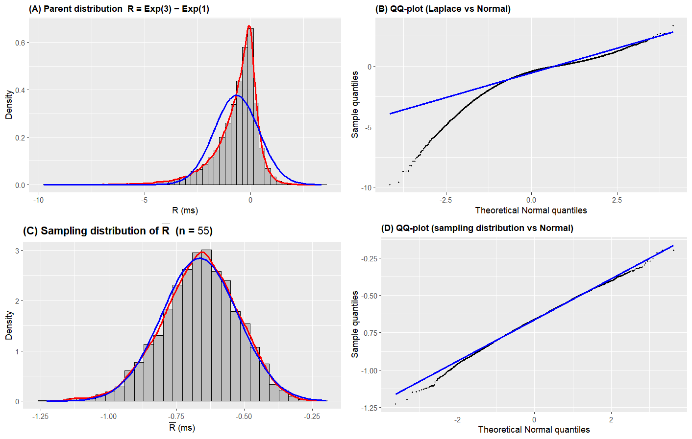
Based on the context of the problem and the plots below (Figures A–D), do you think it is reasonable to approximate \(\bar{R}\) with a Normal distribution using the CLT? Answer yes or no and justify your answer by referring to the characteristics observed in the histograms and QQ-plots.

Solution

Answer: Yes (reasonable) — with caveats.

The parent distribution of \(R\) (Figure A) shows strong left skewness, confirmed by the curved QQ-plot in Figure B where the points deviate substantially from the line. However, for the sample mean \(\bar{R}\) with \(n = 55\) (Figure C), the histogram kernel density and the blue normal overlay are closely aligned, indicating that much of the skewness has been mitigated by averaging. Figure D (QQ-plot of \(\bar{R}\)) shows mostly linear alignment, though some deviation persists in the tails.

The Normal approximation via the CLT is reasonable for most purposes with \(n = 55\). However, if high precision in the tails is required, the approximation may still introduce non-negligible error, since Figure D confirms residual non-normality has not been fully eliminated.

Question 4e (3 pts)

Using the Normal approximation to \(\bar{R}\) with mean \(E[\bar{R}]\) and standard deviation \(\text{SD}(\bar{R})\), select the correct R code to compute the approximate probability \(P(-0.5 \leq \bar{R} \leq 0)\).

• 1. pnorm(0, mean=E[Rbar], sd=SD(Rbar), lower.tail=TRUE) - pnorm(-0.5, mean=E[Rbar], sd=SD(Rbar), lower.tail=FALSE)

• 2. pnorm(0, mean=E[Rbar], sd=SD(Rbar), lower.tail=FALSE) - pnorm(-0.5, mean=E[Rbar], sd=SD(Rbar), lower.tail=TRUE)

• 3. pnorm(0, mean=E[Rbar], sd=SD(Rbar), lower.tail=TRUE) - pnorm(-0.5, mean=E[Rbar], sd=SD(Rbar), lower.tail=TRUE)

• 4. pnorm(0, mean=E[Rbar], sd=SD(Rbar), lower.tail=FALSE) - pnorm(-0.5, mean=E[Rbar], sd=SD(Rbar), lower.tail=FALSE)

Solution

Answer: (C)

The probability of an interval is computed as:

\[P(-0.5 \leq \bar{R} \leq 0) = P(\bar{R} \leq 0) - P(\bar{R} \leq -0.5)\]

Both terms use the CDF (\(\texttt{lower.tail = TRUE}\)), giving:

pnorm(0,   mean = E[Rbar], sd = SD(Rbar), lower.tail = TRUE) -
pnorm(-0.5, mean = E[Rbar], sd = SD(Rbar), lower.tail = TRUE)

• (A) subtracts pnorm(-0.5, ..., lower.tail=FALSE) = \(P(\bar{R} > -0.5)\), which gives a wrong result.

• (B) uses lower.tail=FALSE for the upper limit, yielding \(P(\bar{R} > 0)\), not \(P(\bar{R} \leq 0)\).

• (D) Both terms use lower.tail=FALSE (upper tail), producing \(P(\bar{R}>0) - P(\bar{R}>-0.5)\) which is negative.

—

Problem 5 Setup

Purdue researchers want to establish the relationship between voltage (\(x\), in volts) and the lifetime of semiconductor chips in electric vehicles (\(Y\), in years). They simulated the following data.

Voltage and Chip Lifetime Data

Variable	1	2	3	4	5	6	7	8
Voltage (\(x\), V)	450	812	631	720	364	965	1044	569
Lifetime (\(Y\), years)	17.6	13.4	15.3	14.9	19.7	13.2	12.3	16.8

Problem 5 — Simple Linear Regression (40 points)

Question 5a (3 pts)

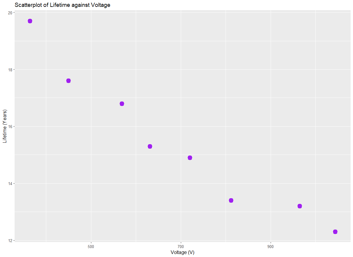
Describe the relationship, strength, and direction of the relationship between lifetime of semiconductor chips and voltage based on the scatter plot below.

Solution

Answer: The relationship between voltage and chip lifetime is linear, with a negative direction and strong (to moderate) association. Higher voltage is associated with shorter chip lifetime.

Question 5b (8 pts)

The following output was obtained from RStudio for the regression fit.

Call:
lm(formula = Lifetime ~ Volt, data = jpr)

Residuals:
     Min       1Q   Median       3Q      Max
-0.80339 -0.40072 -0.05738  0.48086  0.93905

Coefficients:
             Estimate Std. Error t value Pr(>|t|)
(Intercept) 22.463962   0.782290  28.716 1.18e-07 ***
Volt        -0.010173   0.001073  -9.485 7.82e-05 ***
---
Residual standard error: 0.6771 on 6 degrees of freedom
Multiple R-squared:  0.9375,    Adjusted R-squared:  0.9271
F-statistic: 89.96 on 1 and 6 DF,  p-value: 7.824e-05

1. Write out the equation of the regression line.

2. Interpret the meaning of the estimated slope.

3. Find and interpret \(R^2\) in the context of the problem.

Solution

(i) Regression equation:

\[\hat{y} = 22.4640 - 0.0102\,x_{\text{Volt}}\]

(ii) Slope interpretation:

For each additional 1 volt increase in operating voltage, the estimated mean lifetime of a semiconductor chip decreases by approximately 0.0102 years, on average.

(iii) Coefficient of determination:

\(R^2 = 0.9375\). Approximately 93.75% of the variation in the lifetime of semiconductor chips is explained by the linear relationship with voltage. This indicates a very strong linear fit.

Question 5c (12 pts)

Complete the ANOVA table. Show your work.

ANOVA Table for Regression

Source	df	SS	MS	F	\(\Pr(>F)\)
Regression	1	41.249	41.249	89.964	7.824e-05
Error	6	2.751	0.4585
Total	7	44.000

Solution

Degrees of freedom:

\[\text{df}_{\text{Reg}} = 1, \quad \text{df}_E = n - 2 = 8 - 2 = 6, \quad \text{df}_T = n - 1 = 7\]

SST is given directly (= 44).

SSR is given (= 41.249). Cross-check: \(\text{SSR} = F_{\text{TS}} \times \text{MSE} \times \text{df}_{\text{Reg}} = 89.964 \times 0.4585 \times 1 \approx 41.25\) ✓

SSE:

\[\text{SSE} = \text{SST} - \text{SSR} = 44 - 41.249 = 2.751\]

MSE:

\[\text{MSE} = \frac{\text{SSE}}{\text{df}_E} = \frac{2.751}{6} = 0.4585\]

Cross-check: \(\hat{\sigma} = \sqrt{0.4585} = 0.6771\) matches the residual standard error in the output ✓

Question 5d (7 pts)

Based on the ANOVA table, is there a significant linear association between chip lifetime and voltage at \(\alpha = 0.001\)? State the hypotheses and provide a formal conclusion in context.

Solution

Step 1 — Parameter of interest: Let \(\beta_1\) denote the true slope of the linear relationship between voltage (\(x\)) and the mean lifetime of semiconductor chips (\(Y\)).

Step 2 — Hypotheses:

\[H_0\colon \beta_1 = 0 \quad \text{(no linear association between voltage and chip lifetime)}\]

\[H_a\colon \beta_1 \neq 0 \quad \text{(there is a linear association)}\]

Step 3 — Test statistic and p-value:

From the ANOVA table: \(F_{\text{TS}} = 89.964\) on \(\text{df}_M = 1\) and \(\text{df}_E = 6\); \(p\text{-value} = 7.824 \times 10^{-5}\).

Step 4 — Decision and conclusion:

Since \(p\text{-value} = 7.824 \times 10^{-5} < 0.001 = \alpha\), we reject \(H_0\).

The data give support (\(p\)-value \(= 7.824 \times 10^{-5}\)) to the claim that there is a linear relationship between voltage and the lifetime of semiconductor chips in electric vehicles.

Question 5e (10 pts)

Given that \(S_{xx} = 398{,}569.875\), construct a 99.9% confidence interval for \(\beta_1\). Select an appropriate critical value from the R output below.

> qt(0.001, 6, lower.tail = FALSE)
[1] 5.207626
> qt(0.001/2, 6, lower.tail = FALSE)
[1] 5.958816
> qt(0.001, 7, lower.tail = FALSE)
[1] 4.785290
> qt(0.001/2, 7, lower.tail = FALSE)
[1] 5.407883

Solution

Critical value selection:

For a 99.9% two-sided CI, \(\alpha = 0.001\), so we need \(t_{\alpha/2,\,\text{df}_E} = t_{0.0005,\,6}\):

> qt(0.001/2, 6, lower.tail = FALSE)
[1] 5.958816

Standard error of \(\hat{\beta}_1\):

\[\text{SE}(\hat{\beta}_1) = \sqrt{\frac{\text{MSE}}{S_{xx}}} = \sqrt{\frac{0.4585}{398{,}569.875}} = 0.001073\]

(This matches the Std. Error in the R output directly.)

99.9% Confidence interval:

\[\hat{\beta}_1 \pm t_{0.0005,\,6} \cdot \text{SE}(\hat{\beta}_1) = -0.010173 \pm 5.958816 \times 0.001073\]

\[= -0.010173 \pm 0.006394\]

\[\boxed{(-0.0166,\ -0.0038)}\]

Since the interval does not contain zero, this confirms at the 99.9% confidence level that \(\beta_1 < 0\) — higher voltage is associated with shorter chip lifetime.

—

Problem 6 Setup

An ethologist plans to study how vocal cats are when communicating with different species. Five species are selected: humans, dogs, parrots, rabbits, and hamsters. For each species, the duration of vocal communication per week (in minutes) for a group of 20 randomly selected cats is recorded.

Summary Statistics by Species

	Human	Dog	Parrot	Rabbit	Hamster
\(n_i\)	20	20	20	20	20
\(\bar{x}_i\)	50.1	37.4	44.3	15.6	24.3
\(s_i\)	12.3	9.10	10.4	9.35	9.40

Data table note ⚠️

The exam table header labels the last row as \(s_i^2\) (sample variance), but the solution key treats these values as standard deviations \(s_i\) when computing SSE (squaring them to obtain \(s_i^2\)). The F-statistic of 39.038 in the key is consistent only with the standard deviation interpretation. The equal variance check in the key is also consistent with treating these as standard deviations (direct ratio \(s_{\max}/s_{\min}\)). All solutions below follow the key and treat the given values as \(s_i\) (standard deviations).

Problem 6 — One-Way ANOVA (42 points)

Question 6a (3 pts)

When analyzing the data through ANOVA, which of the following statements is TRUE?

• 1. The duration of vocal communication is a factor variable.

• 2. All groups must have the same sample size.

• 3. Measuring time in hours instead of minutes would change the ANOVA results.

• 4. Homogeneity of variance is automatically satisfied because all cats are sampled from the same population.

• 5. None of the above.

Solution

Answer: (E)

• (A) FALSE. The species (Human, Dog, Parrot, Rabbit, Hamster) is the factor variable — it is the categorical grouping variable. The duration of vocal communication is the quantitative response variable.

• (B) FALSE. One-way ANOVA does not require equal group sizes; it accommodates unbalanced designs.

• (C) FALSE. Rescaling the response (minutes → hours, dividing by 60) is a linear transformation that changes all values proportionally. The F-statistic is invariant to such scaling because SSA, SSE, and hence MSA/MSE all scale by the same factor \((1/60)^2\).

• (D) FALSE. Homogeneity of variance refers to the population variance within each group being equal — it must be assessed empirically (e.g., the rule-of-thumb ratio check) and is not guaranteed by sharing a common population.

Question 6b (2 pts)

Check the constant variance assumption using the summary statistics. Show your work and state whether the assumption is satisfied.

Solution

Answer: The equal variance assumption is satisfied.

The rule of thumb checks whether \(s_{\max}/s_{\min} \leq 2\):

\[\frac{s_{\max}}{s_{\min}} = \frac{12.3}{9.10} \approx 1.3516 \leq 2\]

Since the ratio is well below 2, the homogeneity of variance assumption holds.

Question 6c (12 pts)

Complete the ANOVA table. Show your work.

One-Way ANOVA Table

Source	df	SS	MS	F statistic
Factor (Species)	4	16178.64	4044.66	39.0379
Error	95	9842.808	103.6085
Total	99	26021.45

Solution

Degrees of freedom:

\[\text{df}_A = k - 1 = 5 - 1 = 4, \quad \text{df}_E = N - k = 100 - 5 = 95, \quad \text{df}_T = 99\]

Grand mean:

\[\bar{\bar{x}} = \frac{50.1 + 37.4 + 44.3 + 15.6 + 24.3}{5} = \frac{171.7}{5} = 34.34\]

SSA:

\[\text{SSA} = 20\left[(50.1-34.34)^2 + (37.4-34.34)^2 + (44.3-34.34)^2 + (15.6-34.34)^2 + (24.3-34.34)^2\right]\]

\[= 20\left[248.3776 + 9.3636 + 99.2016 + 351.1876 + 100.8016\right] = 20 \times 808.9320 = \mathbf{16{,}178.64}\]

SSE (treating \(s_i\) as standard deviations):

\[\text{SSE} = \sum_{i=1}^{5}(n_i - 1)s_i^2 = 19\!\left(12.3^2 + 9.10^2 + 10.4^2 + 9.35^2 + 9.40^2\right)\]

\[= 19(151.29 + 82.81 + 108.16 + 87.4225 + 88.36) = 19 \times 518.0425 = 9842.808\]

MSA and MSE:

\[\text{MSA} = \frac{16178.64}{4} = 4044.66, \qquad \text{MSE} = \frac{9842.808}{95} = 103.6085\]

F-statistic:

\[F_{\text{TS}} = \frac{\text{MSA}}{\text{MSE}} = \frac{4044.66}{103.6085} \approx 39.0379\]

SST = SSA + SSE = 16178.64 + 9842.808 = 26021.45.

Question 6d (4 pts)

What is the estimated value of the assumed common variance among different species?

Solution

Answer: \(\hat{\sigma}^2 = \text{MSE} = \boxed{103.6085}\)

In one-way ANOVA, the MSE is the pooled estimate of the common within-group variance \(\sigma^2\) (assumed equal across all \(k\) groups under the ANOVA model).

Question 6e (3 pts)

Select the correct R code for the \(p\)-value associated with the ANOVA table. Assume \(F_{\text{TS}}\), \(\text{df}_A\), and \(\text{df}_E\) are the correct test statistic and degrees of freedom.

• 1. pf(FTS, df1 = dfA, df2 = dfE, lower.tail = TRUE)

• 2. pf(FTS, df1 = dfA, df2 = dfE, lower.tail = FALSE)

• 3. 2 * pf(FTS, df1 = dfA, df2 = dfE, lower.tail = FALSE)

• 4. The \(p\)-value cannot be determined without specifying the significance level.

Solution

Answer: (B)

The ANOVA F-test is always upper-tailed: large values of \(F_{\text{TS}}\) indicate evidence against \(H_0\). The \(p\)-value is therefore the probability of observing an F-statistic as large as or larger than the one observed:

\[p\text{-value} = P(F \geq F_{\text{TS}}) = \texttt{pf(FTS, df1 = dfA, df2 = dfE, lower.tail = FALSE)}\]

• (A) gives the CDF value \(P(F \leq F_{\text{TS}})\) — the complement of the p-value.

• (C) doubles the upper tail, which would be appropriate for a two-sided test; F-tests in ANOVA are one-sided.

• (D) is incorrect; the p-value is a computed probability, not dependent on the significance level.

Question 6f (8 pts)

The researchers obtain a \(p\)-value less than \(2 \times 10^{-16}\). At the 1% level of significance, provide a formal decision and conclusion in context.

Solution

Since \(p\text{-value} < 2 \times 10^{-16} < 0.01 = \alpha\), we reject \(H_0\).

The data give support (\(p\)-value \(< 2\times10^{-16}\)) to the claim that the true mean duration of vocal communication per week differs across at least two of the five species studied.

Question 6g (10 pts)

The R output below shows the Tukey HSD results at a family-wise error rate of 5%. Use the output and summary statistics to draw a graphical representation of the Tukey HSD results. Clearly indicate which species (or species, if multiple) has the shortest mean vocal communication duration.

               diff        lwr         upr     p adj
Hamster-Dog  -13.097560 -22.043802  -4.1513175 0.0009019
Human-Dog     12.701642   3.755400  21.6478844 0.0013940
Parrot-Dog     6.912555  -2.033688  15.8587969 0.2085189
Rabbit-Dog   -21.790044 -30.736286 -12.8438015 0.0000000
Human-Hamster 25.799202  16.852960  34.7454442 0.0000000
Parrot-Hamster 20.010114  11.063872  28.9563567 0.0000001
Rabbit-Hamster -8.692484 -17.638726   0.2537583 0.0610890
Parrot-Human   -5.789088 -14.735330   3.1571548 0.3799648
Rabbit-Human  -34.491686 -43.437928 -25.5454436 0.0000000
Rabbit-Parrot -28.702598 -37.648841 -19.7563561 0.0000000

Solution

Graphical representation (underline notation):

Groups connected by the same underline are not significantly different from each other at the 5% family-wise level.

Tukey HSD Groupings

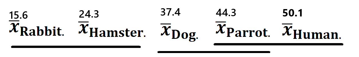
Species	\(\bar{x}_i\)	Significant differences from
Rabbit	15.6	Dog, Human, Parrot (all \(p < 0.001\)); not from Hamster (\(p = 0.061\))
Hamster	24.3	Dog, Human, Parrot (all \(p < 0.01\)); not from Rabbit (\(p = 0.061\))
Dog	37.4	Rabbit, Hamster, Human (all \(p < 0.01\)); not from Parrot (\(p = 0.209\))
Parrot	44.3	Rabbit, Hamster (both \(p < 0.001\)); not from Dog (\(p = 0.209\)) or Human (\(p = 0.380\))
Human	50.1	Rabbit, Hamster, Dog (all \(p < 0.01\)); not from Parrot (\(p = 0.380\))

Conclusion: Rabbit and Hamster are the two species with the shortest mean vocal communication durations in the population. Both are statistically significantly different from every other species (Dog, Parrot, Human), but are not statistically significantly different from each other (\(p\text{-adj} = 0.0611 > 0.05\)). Since their sample means (15.6 and 24.3 minutes/week, respectively) are the two lowest, we conclude that both Rabbit and Hamster elicit the least vocal behavior from cats.