Slides 📊

Download Chapter 9 slides (PPTX)

9.3. Precision of a Confidence Interval

In the previous section, we established that confidence intervals convey the degree of uncertainty through their width. A narrow interval suggests high precision, while a wide interval reflects greater uncertainty. This naturally raises two key questions:

• What factors determine the width of a confidence interval?

• What can we do to make an interval more precise (narrower)?

We will explore the answers to these questions in this lesson.

Road Map 🧭

• Identify the three building blocks of a margin of error and understand how each influences the precision of a confidence interval.

• Understand why the sample size is the only component of an ME that researchers can actively control.

• For a desired level of precision, compute the mininum required sample size, and incorporate this into experiment planning.

9.3.1. What Makes a Confidence Interval Precise?

Fig. 9.5 The width of a confidence interval is equal to 2ME

The width of a confidence interval is entirely determined by its margin of error (ME) as shown in Fig. 9.5. Specifically,

\[\text{width of a CI} = 2ME = 2z_{\alpha/2}\frac{\sigma}{\sqrt{n}}.\]

From its mathematical definition, we can identify three elements that determine the size of an ME: \(\alpha\) (and thus \(C\)), \(\sigma\), and \(n\). Let us examine how each affects the width of a confidence interval.

Component of ME	Effect on precision
Confidence level \(C\)	Higher \(C \to\) the central region of area \(C\) expands \(\to\) \(z_{\alpha/2}\) pushed to the right \(\to\) increased ME & lower precision 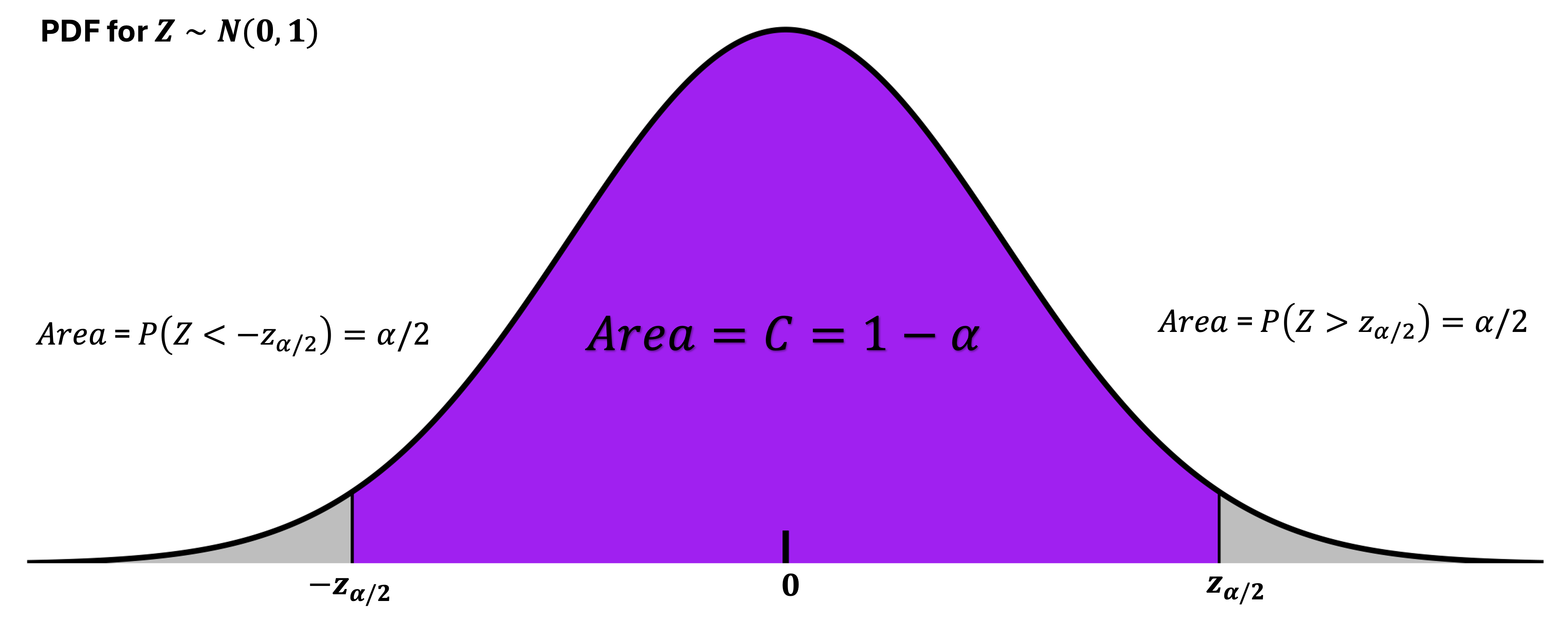Fig. 9.6 Standard normal PDF
Population standard deviation \(\sigma\)	Higher \(\sigma \to\) increaseed ME & lower precision
Sample size \(n\)	Higher \(n \to\) decreased ME & higher precision

Controlling the Precision

Of the three components of a margin of error, researchers can practically control only the sample size, \(n\). The population standard deviation \(\sigma\) is a fixed property of the population, and the confidence level \(C\) must be chosen to reflect the desired rigor of the experiment; it is not meaningful to lower confidence merely to obtain a narrower interval.

This leads to an important practical question: “How do we control the sample size to meet a target precision?”

9.3.2. Sample Size Planning for a Target Precision

Maximum Width

Suppose we want to construct a confidence interval whose width is at most \(w_{max}\). That is, we want

\[\text{width} = 2z_{\alpha/2}\frac{\sigma}{\sqrt{n}} \leq w_{max}.\]

Rearranging to isolate \(n\),

\[\frac{2z_{\alpha/2}\sigma}{w_{max}} \leq \sqrt{n}.\]

Square both sides and bring \(n\) to the left hand side:

\[n \geq \left(\frac{2 z_{\alpha/2} \sigma}{w_{max}}\right)^2.\]

Since \(n\) must be a whole number, we take the the smallest integer on or above the lower bound. That is, the smallest required sample size \(n^*\) for a target width \(w_{max}\) is computed as:

\[n^* = \Bigg\lceil \left(\frac{2 z_{\alpha/2} \sigma}{w_{max}}\right)^2 \Bigg\rceil.\]

Maximum Margin of Error

The desired level of precision can also be given as a maximum margin of error, \(\text{ME}_{max}\). In this case, we take \(n^*\) as:

\[n^* = \Bigg\lceil\left(\frac{z_{\alpha/2} \sigma}{\text{ME}_{max}}\right)^2 \Bigg\rceil\]

through a similar flow of logic. You are encouraged to confirm this result as a quick exercise.

Example 💡: Weights of American Adult Males, Continued

We continue with the study of weights of American male adults from Section 9.2. Suppose the researchers want to compute a 99% confidence interval for the mean weight with a margin of error of at most 1. What is the smallest sample size they need?

The building blocks

• The maximum ME: \(\text{ME}_{max} = 1\).

• The population standard deviation: \(\sigma=49.26\) lbs

• Confidence level: \(99\% \, (C=0.99, \alpha=0.01)\)

• The z-critical value: \(z_{\alpha/2} = z_{0.005} = 2.5758\)

The goal

We would like to compute the smallest integer \(n\) satisfying

\[ME = z_{\alpha/2}\frac{\sigma}{\sqrt{n}} \leq \text{ME}_{max}\]

Rearranging and isolating \(n\),

\[n \geq \left(\frac{z_{\alpha/2}\sigma}{ME_{max}}\right)^2 = \left(\frac{(2.5758)(49.26)}{1}\right)^2 = 16099.53\]

The smallest sample size needed for the desired level of precison is \(n^* = \lceil 16099.53\rceil =16,100\).

9.3.3. Bringing It All Together

Key Takeaways 📝

• The margin of error quantifies the precision of a confidence interval. The three factors of margin of error that control precision are: confidence level \(C\), population variance \(\sigma^2\) (or population sd \(\sigma\)), and sample size \(n\).

• The smallest required sample size for a given maximum ME can be calculated using: \(n^* = \Big\lceil \left(\frac{z_{\alpha/2}\,\sigma}{\text{ME}_{max}}\right)^2\Big\rceil\).

Learning Objectives 🎯

These exercises will help you:

• Identify the three components that determine margin of error

• Understand how each component affects CI precision

• Calculate the minimum sample size for a desired margin of error

• Apply sample size planning to experiment design

• Recognize the diminishing returns of increasing sample size

Key Formulas 📐

Margin of Error:

\[ME = z_{\alpha/2} \frac{\sigma}{\sqrt{n}}\]

Sample Size Formula (for target ME):

\[n^* = \left\lceil \left(\frac{z_{\alpha/2} \cdot \sigma}{ME_{max}}\right)^2 \right\rceil\]

CI Width: \(\text{Width} = 2 \times ME\)

R Function:

# Sample size for target ME
n_star <- ceiling((qnorm(alpha/2, lower.tail=FALSE) * sigma / ME_max)^2)

9.3.4. Exercises

Exercise 1: Components of Margin of Error

The margin of error for a confidence interval when σ is known is \(ME = z_{\alpha/2} \frac{\sigma}{\sqrt{n}}\).

1. List the three components that determine the margin of error.

2. For each component, describe the effect of increasing it on the margin of error (increases, decreases, or no effect).

3. Which component(s) can researchers typically control when planning a study?

4. Why is it generally not appropriate to lower the confidence level just to achieve a narrower interval?

Solution

Part (a): Three components

1. Confidence level \(C\) (through \(z_{\alpha/2}\) where \(\alpha = 1 - C\))

2. Population standard deviation \(\sigma\)

3. Sample size \(n\)

Part (b): Effects of increasing each

• Increasing \(C\): Increases \(z_{\alpha/2}\) → increases ME → wider CI, less precision

• Increasing \(\sigma\): Directly increases ME → wider CI, less precision

• Increasing \(n\): Decreases \(\frac{\sigma}{\sqrt{n}}\) → decreases ME → narrower CI, more precision

Part (c): Controllable components

Researchers directly control sample size \(n\) and choose confidence level \(C\).

• \(\sigma\) is a fixed property of the population (though design choices can sometimes reduce variability)

• \(C\) is chosen based on the desired level of confidence—while it can be lowered to reduce ME, this is generally not appropriate (see part d)

Part (d): Why lowering confidence level is problematic

• It undermines the reliability of the inference

• A narrower interval at lower confidence is “cheap” precision—you’re less certain it contains μ

• The appropriate confidence level should reflect the study’s scientific requirements, not be chosen for convenience

• Reporting a 70% CI just to look more precise would be misleading

---

Exercise 2: Sample Size Calculation - Basic

A materials engineer wants to estimate the hardness of steel samples with a 95% confidence interval. From historical data, the population standard deviation is \(\sigma = 15\) Rockwell units.

Calculate the minimum sample size needed to achieve a margin of error of:

1. ME = 3 Rockwell units

2. ME = 2 Rockwell units

3. ME = 5 Rockwell units

4. What pattern do you notice? How does the required sample size change as the desired precision increases (ME decreases)?

Solution

Given: \(\sigma = 15\) Rockwell units, 95% confidence (\(z_{0.025} = 1.96\))

Formula: \(n^* = \left\lceil \left(\frac{z_{\alpha/2} \cdot \sigma}{ME_{max}}\right)^2 \right\rceil\)

Part (a): ME = 3

\[n^* = \left\lceil \left(\frac{1.96 \times 15}{3}\right)^2 \right\rceil = \left\lceil (9.8)^2 \right\rceil = \left\lceil 96.04 \right\rceil = 97\]

Part (b): ME = 2

\[n^* = \left\lceil \left(\frac{1.96 \times 15}{2}\right)^2 \right\rceil = \left\lceil (14.7)^2 \right\rceil = \left\lceil 216.09 \right\rceil = 217\]

Part (c): ME = 5

\[n^* = \left\lceil \left(\frac{1.96 \times 15}{5}\right)^2 \right\rceil = \left\lceil (5.88)^2 \right\rceil = \left\lceil 34.57 \right\rceil = 35\]

Part (d): Pattern

Desired ME	Required n
5	35
3	97
2	217

As ME decreases (precision increases), the required sample size increases quadratically. Reducing ME from 3 to 2 (a 33% reduction) requires increasing n from 97 to 217 (a 124% increase). Halving ME quadruples the required n.

R verification:

sigma <- 15
z <- qnorm(0.025, lower.tail = FALSE)

ceiling((z * sigma / 3)^2)  # 97
ceiling((z * sigma / 2)^2)  # 217
ceiling((z * sigma / 5)^2)  # 35

---

Exercise 3: Sample Size for CI Width

A pharmaceutical researcher wants to estimate the mean drug concentration in blood samples. The population standard deviation is \(\sigma = 8.4\) ng/mL. The researcher wants a 95% CI with total width no more than 4 ng/mL.

1. What is the maximum margin of error corresponding to a width of 4 ng/mL?

2. Calculate the minimum sample size needed.

3. If the researcher can only afford to collect 50 samples, what would be the resulting CI width?

4. What width could be achieved with 100 samples?

Solution

Given: \(\sigma = 8.4\) ng/mL, 95% confidence (\(z_{0.025} = 1.96\))

Part (a): Maximum ME

Width = 2 × ME, so:

\[ME_{max} = \frac{\text{Width}}{2} = \frac{4}{2} = 2 \text{ ng/mL}\]

Part (b): Minimum sample size

\[n^* = \left\lceil \left(\frac{1.96 \times 8.4}{2}\right)^2 \right\rceil = \left\lceil (8.232)^2 \right\rceil = \left\lceil 67.77 \right\rceil = 68\]

Part (c): CI width with n = 50

\[ME = 1.96 \times \frac{8.4}{\sqrt{50}} = 1.96 \times 1.188 = 2.33 \text{ ng/mL}\]

\[\text{Width} = 2 \times 2.33 = 4.66 \text{ ng/mL}\]

Part (d): CI width with n = 100

\[ME = 1.96 \times \frac{8.4}{\sqrt{100}} = 1.96 \times 0.84 = 1.65 \text{ ng/mL}\]

\[\text{Width} = 2 \times 1.65 = 3.29 \text{ ng/mL}\]

R verification:

sigma <- 8.4
z <- 1.96

# Part (b)
ceiling((z * sigma / 2)^2)  # 68

# Part (c): Width with n = 50
2 * z * sigma / sqrt(50)    # 4.66

# Part (d): Width with n = 100
2 * z * sigma / sqrt(100)   # 3.29

---

Exercise 4: Diminishing Returns

A quality engineer monitors the tensile strength of wire cables with \(\sigma = 25\) N. She wants to understand how sample size affects precision.

1. Complete the table below for a 95% confidence interval:

   Sample Size (n)	Standard Error	Margin of Error	CI Width
   25	?	?	?
   100	?	?	?
   400	?	?	?
   1600	?	?	?

2. Each row quadruples the sample size. By what factor does the CI width decrease each time?

3. What is the practical implication of this pattern for study planning?

Solution

Given: \(\sigma = 25\) N, \(z_{0.025} = 1.96\)

Part (a): Completed table

n	SE = σ/√n	ME = 1.96 × SE	Width = 2 × ME
25	5.00	9.80	19.60
100	2.50	4.90	9.80
400	1.25	2.45	4.90
1600	0.625	1.225	2.45

Part (b): Factor of decrease

Each time n quadruples, the CI width is halved (factor of 2).

This is because \(\text{Width} \propto 1/\sqrt{n}\), and \(\sqrt{4} = 2\).

Part (c): Practical implication

Diminishing returns: To achieve each additional halving of CI width requires quadrupling the sample size. This means:

• Early increases in n are very cost-effective

• Later increases become increasingly expensive relative to the gain in precision

• There’s often a practical “sweet spot” where the cost of additional samples outweighs the marginal improvement in precision

---

Exercise 5: Different Confidence Levels

An aerospace engineer needs to estimate mean thrust with \(\sigma = 500\) N. She wants a margin of error no larger than 100 N.

Calculate the minimum sample size for:

1. 90% confidence

2. 95% confidence

3. 99% confidence

4. Create a table summarizing n, z-critical value, and resulting ME for each confidence level. What tradeoff does this illustrate?

Solution

Given: \(\sigma = 500\) N, \(ME_{max} = 100\) N

Part (a): 90% confidence (\(z_{0.05} = 1.645\))

\[n^* = \left\lceil \left(\frac{1.645 \times 500}{100}\right)^2 \right\rceil = \left\lceil (8.225)^2 \right\rceil = \left\lceil 67.65 \right\rceil = 68\]

Part (b): 95% confidence (\(z_{0.025} = 1.96\))

\[n^* = \left\lceil \left(\frac{1.96 \times 500}{100}\right)^2 \right\rceil = \left\lceil (9.8)^2 \right\rceil = \left\lceil 96.04 \right\rceil = 97\]

Part (c): 99% confidence (\(z_{0.005} = 2.576\))

\[n^* = \left\lceil \left(\frac{2.576 \times 500}{100}\right)^2 \right\rceil = \left\lceil (12.88)^2 \right\rceil = \left\lceil 165.89 \right\rceil = 166\]

Part (d): Summary table and tradeoff

Confidence	z-critical	Required n
90%	1.645	68
95%	1.96	97
99%	2.576	166

Tradeoff: Higher confidence requires larger sample sizes to maintain the same precision. Going from 95% to 99% confidence (a 4 percentage point increase) requires 71% more samples (97 → 166).

---

Exercise 6: Budget Constraints

A clinical researcher has a budget for testing at most 80 patient samples. Each test measures drug clearance rate with \(\sigma = 12\) mL/min.

1. At 95% confidence with n = 80, what margin of error will be achieved?

2. What is the resulting CI width?

3. If the researcher had hoped for ME ≤ 2 mL/min, how many samples would be needed? Is this feasible?

4. What ME could be achieved with a 90% CI using the same n = 80?

Solution

Given: \(\sigma = 12\) mL/min, budget allows n = 80

Part (a): ME with n = 80 at 95% confidence

\[ME = 1.96 \times \frac{12}{\sqrt{80}} = 1.96 \times 1.342 = 2.63 \text{ mL/min}\]

Part (b): CI width

\[\text{Width} = 2 \times 2.63 = 5.26 \text{ mL/min}\]

Part (c): Required n for ME ≤ 2

\[n^* = \left\lceil \left(\frac{1.96 \times 12}{2}\right)^2 \right\rceil = \left\lceil (11.76)^2 \right\rceil = \left\lceil 138.3 \right\rceil = 139\]

Not feasible with budget of 80 samples. Would need 139 samples.

Part (d): ME with 90% CI, n = 80

\[ME = 1.645 \times \frac{12}{\sqrt{80}} = 1.645 \times 1.342 = 2.21 \text{ mL/min}\]

Switching to 90% confidence reduces ME from 2.63 to 2.21 mL/min, but still doesn’t achieve the target of 2.0 mL/min.

---

Exercise 7: Planning a Manufacturing Study

A manufacturing process produces components with \(\sigma = 1.2\) g. An engineer wants a 95% CI with width no more than 0.5 g.

1. Calculate the minimum sample size needed.

2. If the engineer uses systematic sampling by measuring every 10th item off the production line, what potential problem could arise?

3. If each measurement costs $15, what is the minimum budget needed for this precision?

Solution

Given: \(\sigma = 1.2\) g, width ≤ 0.5 g, 95% confidence

Part (a): Required sample size

\(ME_{max} = 0.5/2 = 0.25\) g

\[n^* = \left\lceil \left(\frac{1.96 \times 1.2}{0.25}\right)^2 \right\rceil = \left\lceil (9.408)^2 \right\rceil = \left\lceil 88.51 \right\rceil = 89\]

Part (b): Systematic sampling problem

Measuring every 10th item creates a systematic (non-random) sample. If the production process has any cyclical patterns (e.g., machine warm-up effects, batch variations), this could introduce bias. Random sampling is preferred for valid inference.

If systematic sampling must be used, randomize the starting point (e.g., randomly select a number 1-10 to determine which item to start with), and verify there is no periodicity in the production process that aligns with the sampling interval.

Part (c): Minimum budget

\[\text{Budget} = 89 \times \$15 = \$1,335\]

---

Exercise 8: Unknown σ Planning

When planning a study, σ is often unknown. A researcher estimates σ from a pilot study or uses a conservative estimate.

Suppose a researcher plans to estimate mean reaction time with ME ≤ 10 ms at 95% confidence. Consider three estimates of σ:

• Conservative estimate: σ = 50 ms

• Moderate estimate: σ = 40 ms

• Optimistic estimate: σ = 30 ms

1. Calculate the required sample size for each estimate of σ.

2. If the true σ turns out to be 45 ms and the researcher used the optimistic estimate (σ = 30), what ME will actually be achieved?

3. Why is it often recommended to use a conservative (larger) estimate of σ when planning?

Solution

Given: \(ME_{max} = 10\) ms, 95% confidence (\(z_{0.025} = 1.96\))

Part (a): Required sample sizes

Conservative (σ = 50):

\[n^* = \left\lceil \left(\frac{1.96 \times 50}{10}\right)^2 \right\rceil = \left\lceil (9.8)^2 \right\rceil = 97\]

Moderate (σ = 40):

\[n^* = \left\lceil \left(\frac{1.96 \times 40}{10}\right)^2 \right\rceil = \left\lceil (7.84)^2 \right\rceil = 62\]

Optimistic (σ = 30):

\[n^* = \left\lceil \left(\frac{1.96 \times 30}{10}\right)^2 \right\rceil = \left\lceil (5.88)^2 \right\rceil = 35\]

Part (b): Actual ME if true σ = 45 but used n = 35

\[ME = 1.96 \times \frac{45}{\sqrt{35}} = 1.96 \times 7.606 = 14.9 \text{ ms}\]

The actual ME (14.9 ms) exceeds the target (10 ms) by 49%!

Part (c): Why use conservative estimates

• Using a larger σ estimate leads to a larger sample size

• If the true σ is smaller than estimated, you get better precision than planned (ME < target)

• If the true σ is larger than estimated (as in part b), you fail to meet your precision goal

• It’s better to collect “too many” samples than to end up with insufficient precision

---

Exercise 9: Comparing Precision Requirements

Three different applications require estimating a mean with \(\sigma = 20\):

• Application A: Rough estimate needed; ME ≤ 5 at 90% confidence

• Application B: Moderate precision; ME ≤ 3 at 95% confidence

• Application C: High precision; ME ≤ 1 at 99% confidence

1. Calculate the required sample size for each application.

2. Application C requires how many times more samples than Application A?

3. If each sample costs $50, calculate the cost for each application.

Solution

Given: \(\sigma = 20\)

Part (a): Required sample sizes

Application A (90%, ME ≤ 5): \(z_{0.05} = 1.645\)

\[n_A = \left\lceil \left(\frac{1.645 \times 20}{5}\right)^2 \right\rceil = \left\lceil (6.58)^2 \right\rceil = 44\]

Application B (95%, ME ≤ 3): \(z_{0.025} = 1.96\)

\[n_B = \left\lceil \left(\frac{1.96 \times 20}{3}\right)^2 \right\rceil = \left\lceil (13.07)^2 \right\rceil = 171\]

Application C (99%, ME ≤ 1): \(z_{0.005} = 2.576\)

\[n_C = \left\lceil \left(\frac{2.576 \times 20}{1}\right)^2 \right\rceil = \left\lceil (51.52)^2 \right\rceil = 2654\]

Part (b): Ratio of C to A

\[\frac{n_C}{n_A} = \frac{2654}{44} = 60.3\]

Application C requires about 60 times more samples than Application A.

Part (c): Costs

• Application A: 44 × $50 = $2,200

• Application B: 171 × $50 = $8,550

• Application C: 2654 × $50 = $132,700

---

9.3.5. Additional Practice Problems

True/False Questions (1 point each)

1. Doubling the sample size will halve the margin of error.

   Ⓣ or Ⓕ

2. The population standard deviation σ can be reduced by collecting more samples.

   Ⓣ or Ⓕ

3. To halve the CI width, you must quadruple the sample size.

   Ⓣ or Ⓕ

4. Higher confidence levels require larger sample sizes to maintain the same ME.

   Ⓣ or Ⓕ

5. The sample size formula always gives a whole number.

   Ⓣ or Ⓕ

6. CI width is equal to twice the margin of error.

   Ⓣ or Ⓕ

Multiple Choice Questions (2 points each)

7. If \(\sigma = 10\), what sample size is needed for ME = 2 at 95% confidence?

   Ⓐ 25

   Ⓑ 49

   Ⓒ 97

   Ⓓ 196

8. The sample size formula \(n = \left(\frac{z \sigma}{ME}\right)^2\) shows that n is:

   Ⓐ Directly proportional to ME

   Ⓑ Inversely proportional to ME

   Ⓒ Inversely proportional to ME²

   Ⓓ Independent of ME

9. To decrease ME by a factor of 3 (e.g., from 6 to 2), sample size must increase by a factor of:

   Ⓐ 3

   Ⓑ 6

   Ⓒ 9

   Ⓓ 27

10. Which statement about the ceiling function is correct?

    Ⓐ ⌈67.01⌉ = 67

    Ⓑ ⌈67.99⌉ = 68

    Ⓒ ⌈67.00⌉ = 68

    Ⓓ ⌈67.5⌉ = 67.5

11. A researcher has σ = 15 and wants ME ≤ 3 at 95% confidence. If budget allows only n = 50, the actual ME will be:

    Ⓐ Less than 3

    Ⓑ Exactly 3

    Ⓒ Greater than 3

    Ⓓ Cannot be determined

12. The “diminishing returns” principle means:

    Ⓐ Larger samples always give the same ME

    Ⓑ Each additional sample contributes less to precision than the previous one

    Ⓒ Sample size has no effect on CI width

    Ⓓ Higher confidence gives narrower intervals

Answers to Practice Problems

True/False Answers:

1. False — Doubling n reduces ME by factor of √2 ≈ 1.41, not 2.

2. False — σ is a fixed population property; it cannot be changed by sampling.

3. True — Width ∝ 1/√n, so halving width requires n × 4.

4. True — Higher confidence means larger z-critical value, requiring more samples for same ME.

5. False — The formula often gives non-integers; we round up (ceiling function).

6. True — CI is x̄ ± ME, so width = (x̄ + ME) − (x̄ − ME) = 2ME.

Multiple Choice Answers:

7. Ⓒ — n = ⌈(1.96 × 10/2)²⌉ = ⌈96.04⌉ = 97.

8. Ⓒ — n = (zσ/ME)² means n ∝ 1/ME².

9. Ⓒ — If ME decreases by factor of 3, n increases by 3² = 9.

10. Ⓑ — Ceiling rounds up to the nearest integer, so ⌈67.99⌉ = 68.

11. Ⓒ — Required n = 97, but only 50 available. ME = 1.96 × 15/√50 = 4.16 > 3.

12. Ⓑ — As n increases, the marginal improvement in precision decreases.