Slides 📊

• Hypothesis Testing for Single Sample (Part 3) (PPTX)

10.3. Connecting CI and HT; t-Test for μ When σ Is Unknown

Hypothesis testing and confidence regions are complementary tools that address essentially the same question from two different perspectives. When certain conditions are carefully matched, a confidence region and a hypothesis test yield outcomes that carry direct implications for one another.

We also dicsuss how to extend our understanding of hypothesis testing to cases where the population standard deviation is unknown. As with confidence regions, we employ the \(t\)-distribution to construct a testing procedure that accounts for the added uncertainty.

Road Map 🧭

• Understand the underlying connection between confidence regions and hypothesis testing. For a given confidene region, identify its complementary hypothesis testing scenario, and vice versa.

• Use the \(t\)-distribution to construct hypothesis tests when the population standard deviation \(\sigma\) is unknown.

10.3.1. The Duality of Hypothesis Tests and Confidence Regions

Two Perspectives on the Same Question

We begin our discussion by comparing the key components of hypothesis testing and confidence regions:

Inference Component	Confidence region for \(\mu\)	Hypothesis testing on \(\mu\)
Parameter of interest	They both aim to understand a population mean, \(\mu\)
Question	“What parameter values are consistent with the sample?”	“Is this specific parameter value consistent with the sample?”
How inference strength is conveyed	A large \(C\)	A small \(\alpha\)
Sample information used	Both use \(\bar{X}\) and its approximate normality due to the CLT
Outcome	A range of plausible values	Answer to whether a candidate value (\(\mu_0\)) is plausible

It is evident from the summary above that confidence intervals and hypothesis tests address the same fundamental question from different angles.

The mathematical connection becomes even deeper when the two inference methods are matched by their inferential strengths and sidedness. Under this pairing, the two methods are in fact equivalent: the result of one has direct implications for the result of the other.

Confidence Intervals and Two-sided Hypothesis Tests

Consider the \(C \cdot 100 \%\) confidence interval for a population mean. With \(\alpha=1-C\), we use the formula:

\[\left(\bar{x} - z_{\alpha/2} \frac{\sigma}{\sqrt{n}}, \bar{x} + z_{\alpha/2} \frac{\sigma}{\sqrt{n}}\right).\]

Let us now perform a two-sided hypothesis test on a candidate value \(\mu_0\) using the significance level \(\alpha = 1-C\). The hypotheses are:

\[\begin{split}&H_0: \mu = \mu_0\\ &H_a: \mu \neq \mu_0\end{split}\]

Based on the cutoff method, we reject the null hypothesis if:

\[\bar{x} \geq z_{\alpha/2}\frac{\sigma}{\sqrt{n}} + \mu_0 \quad \text{ or } \quad \bar{x} \leq -z_{\alpha/2}\frac{\sigma}{\sqrt{n}} + \mu_0.\]

Isolate \(\mu_0\) in both inequalities. Then the null hypothesis is rejected when:

\[\bar{x} - z_{\alpha/2}\frac{\sigma}{\sqrt{n}} \geq \mu_0 \quad \text{ or } \quad \bar{x} + z_{\alpha/2}\frac{\sigma}{\sqrt{n}} \leq \mu_0.\]

Note that the left-hand side of the inequalities are exactly the two ends of the confidence interval.

The Connection

The null hypothesis for a two-tailed test is rejected excatly when the null value \(\mu_0\) is outside a matching confidence interval. Conversely, if the chosen \(\mu_0\) is inside the confidence interval, we would not reject the null hypothesis for that test.

Lower Confidence Bounds and Upper-Tailed Tests

The \(C\cdot 100 \%\) lower confidence bound for the population mean \(\mu\) is:

\[\left(\bar{x} - z_{\alpha} \frac{\sigma}{\sqrt{n}}, \quad \infty\right).\]

When performing an upper-tailed test:

\[\begin{split}&H_0: \mu \leq \mu_0\\ &H_a: \mu > \mu_0,\end{split}\]

we reject the null hypothesis if \(\bar{x} \geq z_\alpha\frac{\sigma}{\sqrt{n}} + \mu_0\). By isolating \(\mu_0\), the inequality becomes:

\[\bar{x} - z_\alpha\frac{\sigma}{\sqrt{n}} \geq \mu_0.\]

The Connection

Given \(\alpha = 1-C\), the null hypothesis of an upper-tailed test is rejected if and only if the null value \(\mu_0\) fails to be inside the confidence region defined by the lower bound.

Upper Confidence Bounds and Lower-Tailed Tests

The \(C\cdot 100 \%\) upper confidence bound for the population mean \(\mu\) is:

\[\left(-\infty, \quad \bar{x} + z_{\alpha} \frac{\sigma}{\sqrt{n}} \right).\]

For a lower-tailed hypothesis test with

\[\begin{split}&H_0: \mu \geq \mu_0\\ &H_a: \mu < \mu_0,\end{split}\]

The null hypothesis is rejected if \(\bar{x} \leq -z_\alpha\frac{\sigma}{\sqrt{n}} + \mu_0\). By isolating \(\mu_0\), the inequality becomes:

\[\bar{x} + z_\alpha\frac{\sigma}{\sqrt{n}} \leq \mu_0.\]

The Connection

As expected, the values of \(\mu_0\) that lead to rejection of the null hypothesis in a lower-tailed test coincide with those that fall outside the upper confidence bound of a matching confidence level, \(C= 1-\alpha\).

Summary

For the duality to work, we need three crucial conditions:

1. The two inference methods are being applied to the same experimental result.

2. \(C + \alpha = 1\).

3. The methods are paired corrrectly based on sidedness (two-sided test and CI, upper-tailed test and LCB, lower-tailed test and UCB).

When these conditions hold,

• \(\mu_0\) lies inside the confidence region \(\iff\) fail to reject \(H_0\)

• \(\mu_0\) lies outside the confidence region \(\iff\) reject \(H_0\)

Example 💡: Quality Control for Cherry Tomatoes

Tom Green oversees quality control for a large produce company. The weights of cherry tomato packages are known to be normally distributed with \(\mu=227g\) (1/2 lbs) and \(\sigma=5g\). He obtains a simple random sample of four packages of cherry tomatoes and discovers that their average weight is 222g.

1. Construct a 95% confidence interval for the mean weight.

2. Tom would like to test whether the true mean weight of the packages is different from 227g with \(\alpha = 0.05\). Based on the result of #1, (do not compute the test statistic or the \(p\)-value), predict wether the null hypothesis will be rejected.

3. Perform the hypothesis test and confirm your answer from part 2.

Q1: Construct the 95% Confidence Interval

Since \(\sigma\) is known and the data is normally distributed, we use the \(z\)-procedure. In general,

\[\left(\bar{x} - z_{\alpha/2} \frac{\sigma}{\sqrt{n}}, \bar{x} + z_{\alpha/2} \frac{\sigma}{\sqrt{n}}\right).\]

For 95% confidence, \(\alpha = 0.05\). The critical value \(z_{0.025}\) can be found using:

z_critical <- qnorm(0.025, lower.tail = FALSE)
z_critical
# [1] 1.959964

Calculate the interval:

\[\left(222 - (1.96)\frac{5}{\sqrt{4}}, 222 + (1.96) \frac{5}{\sqrt{4}}\right) = (217.1, 226.9)\]

We are 95% confident that the true mean weight of cherry tomato packages is captured between 217.1 and 226.9 grams.

Q2: Use Duality to Predict the Conlusion for the Hypothesis Test

We want to test:

\[\begin{split}&H_0: \mu = 227\\ &H_a: \mu \neq 227\end{split}\]

Since we have \(C + \alpha = 0.95 + 0.05 = 1\), and both the confidence region and the hypothesis test are two-sided, the duality relationship applies. The null value \(\mu_0 = 227\) lies outside the 95% confidence interval \((217.1, 226.9)\). Therefore, we would reject the null hypothesis if we performed the hypothesis test. \(\mu_0 = 227\) is NOT a plausaible value for the true mean weight according to the CI, so we should be able to draw the same conclusion from the dual hypothesis test.

Q3: Verify with Formal Hypothesis Test

Let’s confirm this conclusion by performing a z-test for the hypothesis pair.

\[z_{TS} = \frac{\bar{x} - \mu_0}{\sigma/\sqrt{n}} = \frac{222 - 227}{5/\sqrt{4}} = \frac{-5}{2.5} = -2.0\]

The p-value is:

z_test_stat <- -2.0
p_value <- 2 * pnorm(abs(z_test_stat), lower.tail = FALSE)
p_value
# [1] 0.04550026

Since p-value = \(0.0455 < \alpha = 0.05\), we reject the null hypothesis. Both approaches give the same conclusion. This confirms the duality relationship.

10.3.2. \(t\)-Tests: When σ is Unknown

So far, we have been building our test procedures based on the convenient assumption that the population standard deviation is known. If we do not know the population mean \(\mu\), however, we almost certainly do not know \(\sigma\), either.

In such cases, we will take the natural step of replacing the unknown \(\sigma\) with the estimator, \(S\). The sample standard deviation \(S\) is itself a random variable that varies from sample to sample, and this extra variability must be accounted for.

The Assumptions

For the new test procedure, we use a slightly modified set of assumtions:

1. \(X_1, X_2, \cdots, X_n\) form an iid sample from the population \(X\) with mean \(\mu\) and variance \(\sigma^2\).

2. Either the population \(X\) is normally distributed, or the sample size \(n\) is sufficiently large for the CLT to hold.

3. The population variance \(\sigma^2\) is unknown.

The only difference is that the population variance (and sd) is unknown.

The \(t\)-Test Statistic

Recall that when \(\sigma\) was known, the \(z\)-test statistic

\[Z_{TS} = \frac{\bar{X}-\mu_0}{\sigma/\sqrt{n}}\]

played a key role. We used it to

• measure the standardized discrepancy of the data from the null assumption,

• compare it with a \(z\)-critical value and draw a conclusion using the cutoff method, and

• compute the tail probabiltiy of the observed \(z_{TS}\) and draw a conclusion in the \(p\)-value method.

We obtain a new test statistic by replacing the ununknown \(\sigma\) with the sample standard deviation, \(S:\)

\[T_{TS} = \frac{\bar{X} - \mu_0}{S/\sqrt{n}}\]

This new test stastistic is called the \(t\)-test statistic. When the null hypothesis holds, the \(t\)-test statistic has a \(t\)-distribution with the degrees of freedom \(\nu= n-1\).

The \(t\)-test statistic plays the same roles as the \(z\)-test statistic, but we must account for the change in distribution by referencing the appropriate t-distribution rather than standard normal when computing critical values and \(p\)-values.

Cutoff Method for \(t\)-Tests

Recall that the cutoff method rejects the null hypothesis if the observed test statistic falls in a region that is too unusual for the null hypothesis.

For an upper-tailed \(t\)-test, the null hypothesis would be rejected if the observed sample mean is much higher than the null value \(\mu_0\) and satisfies:

\[t_{TS} = \frac{\bar{x}-\mu_0}{s/\sqrt{n}} > t_{\alpha, n-1},\]

where \(t_{\alpha, n-1}\) is the appropriate \(t\)-critical value.

Likewise, the rejection rule for a lower-tailed test is:

\[t_{TS} = \frac{\bar{x}-\mu_0}{s/\sqrt{n}} < -t_{\alpha, n-1}.\]

Finally, for a two-tailed test,

\[|t_{TS}| = \left|\frac{\bar{x}-\mu_0}{s/\sqrt{n}}\right| > t_{\alpha/2, n-1}.\]

\(p\)-Values for \(t\)-Tests

\(p\)-Values for \(t\)-Tests
Upper-tailed p-value	\[P(T_{n-1} \geq t_{TS})\] tts <- (xbar-mu0)/(s/sqrt(n)) pt(tts, df=n-1, lower.tail=FALSE)
Lower-tailed p-value	\[P(T_{n-1} \leq t_{TS})\] pt(tts, df=n-1)
Two-tailed p-value	\[2P(T_{n-1} \leq -|t_{TS}|) \quad \text{ or } \quad 2P(T_{n-1} \geq |t_{TS}|)\] 2 * pt(-abs(tts), df=n-1) 2 * pt(abs(tts), df=n-1, lower.tail=FALSE)

The Rejection Rule Remains Unchanged

Once a \(p\)-value is computed, it is compared against a pre-specified significance level \(\alpha\). If the \(p\)-value is less than \(\alpha\), the null hypothesis is rejected.

Example 💡: Radon Detector Accuracy

University researchers want to find out whether their radon detectors are working correctly. Thy collected a random sample of 12 detectors and placed them in a chamber exposed to exactly 105 picocuries per liter of radon. If the detectors work properly, their measurements should be close to 105, on average.

The Measurements (in picocuries per liter)
91.9	97.8	111.4	122.3	105.4	95.0
103.8	99.6	119.3	104.8	101.7	96.6

In addition, suppose that the population distribution is known to be normal. Perform a hypothesis test with the significance level \(\alpha=0.1\).

Step 0: Which Procedure?

The experiment uses a random sample from a normally distributed population. Therefore, we are justified to use an inference method which assumes approximate normality of the sample mean. We use the \(t\)-test procedure since the population standard deviation is unknown.

Step 1: Define the Parameter

Let \(\mu\) denote the true mean of the measurements produced by the detectors in a chamber with exactly 105 picocuries per liter of radon.

Step 2: State the Hypotheses

\[\begin{split}&H_0: \mu = 105\\ &H_a: \mu \neq 105\end{split}\]

Step 3: Calculate the Observed Test Statistic and the p-value

Comonents:

• \(n=12\)

• \(\bar{x}=104.1333\)

• \(s = 9.397421\)

• \(df = n-1 = 11\)

The sample mean and the sample standard deviation can be computed from the data set.

\[t_{TS} = \frac{\bar{x} - \mu_0}{s/\sqrt{n}} = \frac{104.1333 - 105}{9.397421/\sqrt{12}} = \frac{-0.8667}{2.7136} = -0.319\]

The \(p\)-value is computed using R:

p_value <- 2 * pt(abs(t_test_stat), df = 11, lower.tail = FALSE)
p_value
# [1] 0.755

Step 4: Make the Decision and Write the Conclusion

Since \(p\)-value \(= 0.755 > \alpha = 0.10\), we fail to reject the null hypothesis. With the significance level \(\alpha=0.1\), we do not have enough evidence to reject the null hypothesis that the true mean measurent is 105 picocuries per liter.

🤔 Why Such a Large P-Value?

Although the individual measurements in the data set seem quite inaccurate, we failed to reject the null hypothesis with a large \(p\)-value of \(0.755\). Several factors contribute:

1. The sample mean (\(\bar{x} = 104.1\)) is very close to null value (\(\mu_0 = 105.0\)).

2. The sample size of 12 is small and limits precision.

3. The sample standard deviation (\(s=9.4\)) is relatively large.

4. We are performing a two-sided test, which makes the rejection region farther toward the tails than a one-sided test.

This example illustrates why, in hypothesis testing, we say we “fail to reject” rather than “accept” the null hypothesis. The absence of evidence against the null does not necessarily constitute evidence in its favor.

When there is a large degree of uncertainty, hypothesis tests tend to grow more conservative, which means that it will require the evidence to be stronger for a rejection of the null.

Duality Revisited for \(t\)-Procedures

The duality relationship established for \(z\)-procedures carries over directly to \(t\)-procedures. A confidence region and a hypothesis test based on \(t\)-distributions are equivalent if:

1. The two inference methods are being applied to the same experimental result.

2. \(C + \alpha = 1\).

3. The methods are paired corrrectly based on sidedness (two-sided test and CI, upper-tailed test and LCB, lower-tailed test and UCB).

Example 💡: Complementary CI for Radon Detector Accuracy

Compute the 90% confidence interval for the Radon Detector experiment and comment on its consistency with the hypothesis test.

A \(t\)-confidence interval is, in general,

\[\left(\bar{x} - t_{\alpha/2, n-1}\frac{s}{\sqrt{n}}, \quad \bar{x} + t_{\alpha/2, n-1}\frac{s}{\sqrt{n}}\right).\]

From the previous example, we have:

• \(\bar{x} =104.1333\)

• \(s = 9.397421\)

• \(n = 12\)

The t-critical value \(t_{\alpha/2, n-1}\) is computed using R:

alpha <- 0.10
t_critical <- qt(alpha/2, df = 11, lower.tail = FALSE)
t_critical
# [1] 1.795885

Substituting the values to the general formula, the 90% confidence interval is:

\[(99.3, 109.0).\]

Since \(\mu_0 = 105\) lies within this interval, the duality principle tells us we should fail to reject \(H_0\), which matches our hypothesis test conclusion.

Single-call Verification Using t.test

When the raw data set is available, the R command t.test produces both inference results simultaneously.

radon <- c(91.9, 97.8, 111.4, 122.3, 105.4,
     95.0, 103.8, 99.6, 119.3, 104.8, 101.7, 96.6)

t.test(radon,
       mu = 105,
       alternative = "two.sided",
       conf.level=0.9)

#output
'''
One Sample t-test

data:  radon

t = -0.31947, df = 11, p-value = 0.7554
alternative hypothesis: true mean is not equal to 105

90 percent confidence interval:
99.26145 109.00521

sample estimates:
mean of x
104.1333
'''

The \(t\)-statistic, \(p\)-value, and confidence interval match the hand calculations—always a good final check.

10.3.3. \(t\)-Procedures vs. \(z\)-Procedures

We learned in Chapter 9.5.4 that for any given significance level, the \(t\)-critical value decreases as \(n\) (and therefore the df) increases. This also meant that

\[t_{\alpha, n-1} > z_\alpha\]

for any finite \(n\), since the standard normal distribution can be viewed as a \(t\)-distribution with “infinite” degrees of freedom. As a result, \(t\)-based confidence regions were wider on average than \(z\)-based regions.

In hypothesis tests, if the observed test statistic is held constant, its p-value is larger in a \(t\)-test than in a \(z\)-test because the tails of a \(t\)-distribution are heavier than those of the standard normal. This makes it more difficult for a \(t\)-test to reject the null hypothesis.

The trend is consistent: in the presence of added uncertainty, both inference methods become more conservative—more cautious in labeling an experimental result as unusual. The confidence region widens, and the test becomes more reluctant to reject the status quo.

10.3.4. Bringing It All Together

Key Takeaways 📝

1. Hypothesis tests and confidence regions are dual procedures that address the same questions from different perspectives, connected by the relationship \(C + \alpha = 1\). Further,

   • Two-sided hypothesis tests pair with confidence intervals.

   • Upper-tailed tests pair with lower confidence bounds.

   • Lower-tailed tests pair with upper confidence bounds.

2. When the population standard deviation \(\sigma\) is unknown, \(t\)-tests are used instead of \(z\)-tests.

3. \(t\)-procedures generally produce more conservative inference results than the corresponding \(z\)-procedure; the confidence regions are wider, and it is more difficult to reject the null hypothesis.

10.3.5. Exercises

Exercise 1: T vs Z Critical Values

Compare t-critical values to z-critical values for a two-tailed test at α = 0.05.

1. Find \(z_{0.025}\) (standard normal).

2. Find \(t_{0.025, df}\) for df = 5, 10, 20, 30, 100.

3. Create a table comparing these values.

4. What pattern do you observe as df increases?

5. Explain why t-critical values are larger than z-critical values.

Solution

Part (a): Z-critical value

\(z_{0.025} = 1.960\)

Parts (b) and (c): T-critical values and comparison

df	\(t_{0.025, df}\)	Difference from z
5	2.571	+0.611
10	2.228	+0.268
20	2.086	+0.126
30	2.042	+0.082
100	1.984	+0.024
∞ (z)	1.960	0

Part (d): Pattern

As df increases, t-critical values decrease and approach the z-critical value. By df = 30, the difference is small (~0.08). By df = 100, they’re nearly identical.

Part (e): Why t > z

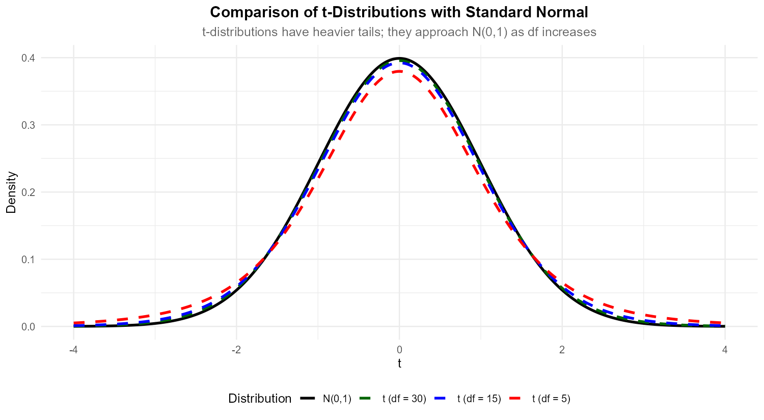
Fig. 10.24 The t-distribution has heavier tails than the standard normal, especially with low df.

T-critical values are larger because the t-distribution has heavier tails than the standard normal. This reflects the additional uncertainty from estimating σ with s—we “pay a penalty” for not knowing the true σ. More probability mass in the tails means we must go further from the center to capture the same probability.

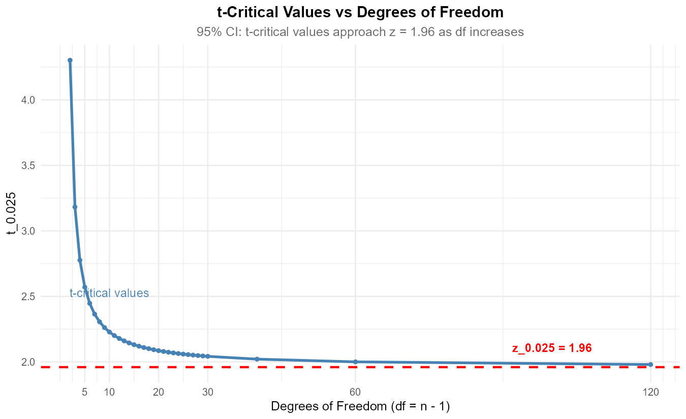
Fig. 10.25 As df → ∞, t-critical values converge to z-critical values.

R verification:

qnorm(0.025, lower.tail = FALSE)  # 1.960
qt(0.025, df = 5, lower.tail = FALSE)   # 2.571
qt(0.025, df = 10, lower.tail = FALSE)  # 2.228
qt(0.025, df = 20, lower.tail = FALSE)  # 2.086
qt(0.025, df = 30, lower.tail = FALSE)  # 2.042
qt(0.025, df = 100, lower.tail = FALSE) # 1.984

---

Exercise 2: Computing T-Test Statistics

Calculate the t-test statistic and state the degrees of freedom for each scenario.

1. \(\bar{x} = 24.5\), \(\mu_0 = 22\), \(s = 5.2\), \(n = 16\)

2. \(\bar{x} = 98.3\), \(\mu_0 = 100\), \(s = 4.1\), \(n = 12\)

3. \(\bar{x} = 515\), \(\mu_0 = 500\), \(s = 45\), \(n = 25\)

Solution

Formula: \(t_{TS} = \frac{\bar{x} - \mu_0}{s / \sqrt{n}}\), df = n - 1

Part (a):

\[t_{TS} = \frac{24.5 - 22}{5.2 / \sqrt{16}} = \frac{2.5}{1.3} = 1.923\]

df = 16 - 1 = 15

Part (b):

\[t_{TS} = \frac{98.3 - 100}{4.1 / \sqrt{12}} = \frac{-1.7}{1.184} = -1.436\]

df = 12 - 1 = 11

Part (c):

\[t_{TS} = \frac{515 - 500}{45 / \sqrt{25}} = \frac{15}{9} = 1.667\]

df = 25 - 1 = 24

---

Exercise 3: P-values with T-Distribution

Calculate p-values for each scenario from Exercise 2.

1. Part (a) data: Upper-tailed test (Hₐ: μ > 22)

2. Part (b) data: Two-tailed test (Hₐ: μ ≠ 100)

3. Part (c) data: Upper-tailed test (Hₐ: μ > 500)

4. Compare these p-values to what you would get using z-distribution. Which are larger?

Solution

Part (a): t = 1.923, df = 15, upper-tailed

\[p\text{-value} = P(T_{15} > 1.923) = 0.0369\]

Part (b): t = -1.436, df = 11, two-tailed

\[p\text{-value} = 2 \times P(T_{11} > 1.436) = 2 \times 0.0894 = 0.1788\]

Part (c): t = 1.667, df = 24, upper-tailed

\[p\text{-value} = P(T_{24} > 1.667) = 0.0543\]

Part (d): Comparison with z-distribution

Using z instead of t:

• 1. P(Z > 1.923) = 0.0272 (t gives 0.0369)

• 2. 2 × P(Z > 1.436) = 0.151 (t gives 0.179)

• 3. P(Z > 1.667) = 0.0478 (t gives 0.0543)

T-distribution p-values are always larger because the t-distribution has heavier tails. This makes it harder to reject H₀ with a t-test, appropriately accounting for the uncertainty in estimating σ.

R verification:

# T-distribution p-values
pt(1.923, df = 15, lower.tail = FALSE)     # 0.0369
2 * pt(abs(-1.436), df = 11, lower.tail = FALSE)  # 0.1788
pt(1.667, df = 24, lower.tail = FALSE)     # 0.0543

# Z-distribution p-values (for comparison)
pnorm(1.923, lower.tail = FALSE)  # 0.0272

---

Exercise 4: Checking Assumptions Before a T-Test

Before conducting a one-sample t-test, we must verify that key assumptions are satisfied. The validity of our inference depends on these assumptions being reasonably met.

A biomedical engineer measures the response time (ms) of a neural signal processing chip for n = 15 test signals:

12.4, 14.2, 11.8, 15.1, 13.5, 12.9, 14.7, 11.2, 13.8, 12.1,
14.5, 13.2, 15.8, 12.6, 13.9

The manufacturer claims the chip has a mean response time of 12.0 ms. Before testing this claim, assess whether the assumptions are satisfied.

Diagnostic Plots:

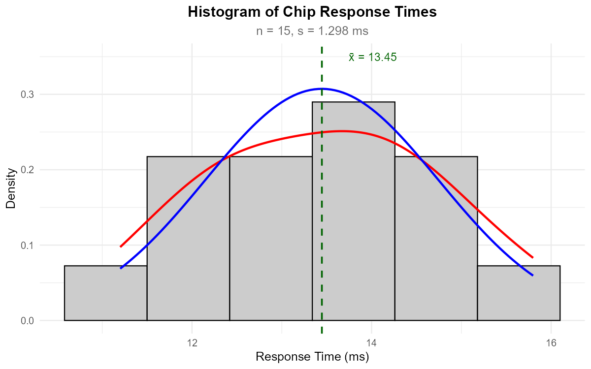
Fig. 10.26 Histogram with kernel density (red) and normal overlay (blue)

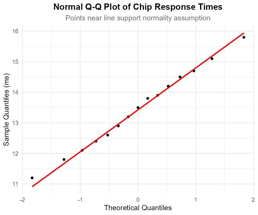
Fig. 10.27 Normal Q-Q plot

1. What are the assumptions required for a valid one-sample t-test?

2. Based on the histogram, does the data appear approximately normal? Comment on symmetry and shape.

3. Based on the QQ-plot, does the normality assumption appear satisfied? Explain what to look for.

4. If normality were severely violated and n remained at 15, what would you recommend?

5. If the sample size were n = 50, would the normality check be as critical? Explain using the Central Limit Theorem.

6. Assuming the assumptions are satisfied, conduct the hypothesis test at α = 0.05 using the complete four-step framework.

Solution

Part (a): Assumptions for one-sample t-test

1. Random sampling / Independence: The observations must be independent and randomly selected from the population.

2. Normality: The population from which the sample is drawn should be approximately normally distributed, OR the sample size should be large enough (n ≥ 30) for the Central Limit Theorem to apply.

Part (b): Histogram assessment

The histogram shows:

• Shape: Approximately symmetric and unimodal

• Center: The distribution is centered around 13-14 ms

• Spread: Reasonable spread without extreme outliers

• Comparison to normal: The kernel density (red) and normal overlay (blue) track each other reasonably well

Assessment: The histogram supports approximate normality ✓

Part (c): QQ-plot assessment

In a QQ-plot, we look for:

• Points falling approximately along the reference line

• No systematic curvature (S-shape suggests skewness, U-shape suggests heavy tails)

• No extreme departures in the tails

The QQ-plot shows points closely following the reference line with minor random deviations expected for n = 15. There is no systematic pattern suggesting departure from normality.

Assessment: The QQ-plot supports approximate normality ✓

Part (d): If normality were severely violated

With n = 15 (small sample) and severe non-normality, options include:

1. Transform the data (e.g., log transformation if right-skewed)

2. Use a nonparametric test such as the Wilcoxon signed-rank test (beyond STAT 350 scope)

3. Increase sample size to invoke the CLT

4. Report cautiously that results may not be reliable

Do NOT proceed with the t-test if assumptions are severely violated.

Part (e): Effect of larger sample size (CLT)

With n = 50, the normality check becomes less critical because:

• The Central Limit Theorem states that for sufficiently large n, the sampling distribution of x̄ is approximately normal regardless of the population distribution

• The general guideline is n ≥ 30, though this depends on the severity of non-normality

• With n = 50, we can be confident the sampling distribution of x̄ is approximately normal even if the underlying data shows moderate skewness or non-normality

Key insight: The normality assumption is about the sampling distribution of x̄, not the raw data. Large samples ensure x̄ is approximately normal via CLT.

Part (f): Complete hypothesis test

First, calculate summary statistics:

times <- c(12.4, 14.2, 11.8, 15.1, 13.5, 12.9, 14.7, 11.2, 13.8, 12.1,
           14.5, 13.2, 15.8, 12.6, 13.9)
n <- length(times)   # 15
xbar <- mean(times)  # 13.447
s <- sd(times)       # 1.278

Step 1: Define the parameter

Let μ = true mean response time (ms) of the neural signal processing chip.

Step 2: State the hypotheses

\[H_0: \mu = 12.0 \quad \text{vs} \quad H_a: \mu \neq 12.0\]

In words: H₀ states the mean response time equals the claimed 12.0 ms. Hₐ states the mean response time differs from 12.0 ms.

Step 3: Check assumptions and calculate test statistic

Assumption checks:

• Independence: Assumed satisfied by the experimental design (separate test signals)

• Normality: With n = 15 (< 30), normality must be verified. The histogram and QQ-plot both support approximate normality ✓

Test statistic:

\[t_{TS} = \frac{\bar{x} - \mu_0}{s / \sqrt{n}} = \frac{13.447 - 12.0}{1.278 / \sqrt{15}} = \frac{1.447}{0.330} = 4.385\]

Degrees of freedom: df = n - 1 = 14

P-value (two-tailed):

\[p\text{-value} = 2 \times P(T_{14} > 4.385) = 0.00063\]

Step 4: Decision and Conclusion

Since p-value = 0.00063 < α = 0.05, reject H₀.

Conclusion: At the 0.05 significance level, there is sufficient evidence to conclude that the true mean response time of the chip differs from the manufacturer’s claim of 12.0 ms (p < 0.001). The sample mean of 13.45 ms suggests the chip is actually slower than claimed.

R verification:

times <- c(12.4, 14.2, 11.8, 15.1, 13.5, 12.9, 14.7, 11.2, 13.8, 12.1,
           14.5, 13.2, 15.8, 12.6, 13.9)

# Verify summary statistics
mean(times)  # 13.447
sd(times)    # 1.278

# Conduct t-test
t.test(times, mu = 12, alternative = "two.sided")

# Output confirms:
# t = 4.385, df = 14, p-value = 0.000628
# 95% CI: (12.74, 14.16)

---

Exercise 5: Complete T-Test (Upper-tailed)

A battery manufacturer claims their new batteries last more than 20 hours on average. A consumer group tests n = 16 batteries and finds \(\bar{x} = 22.1\) hours with s = 4.2 hours. Test the manufacturer’s claim at α = 0.05.

Perform a complete hypothesis test using the four-step framework.

Solution

Step 1: Define the Parameter

Let μ = true mean battery life (hours).

Step 2: State the Hypotheses

\[H_0: \mu \leq 20 \quad \text{vs} \quad H_a: \mu > 20\]

Step 3: Calculate Test Statistic and P-value

Since σ is unknown, use t-test.

\[t_{TS} = \frac{22.1 - 20}{4.2 / \sqrt{16}} = \frac{2.1}{1.05} = 2.00\]

df = 16 - 1 = 15

P-value (upper-tailed):

\[p\text{-value} = P(T_{15} > 2.00) = 0.0320\]

Step 4: Decision and Conclusion

Since p-value = 0.0320 < α = 0.05, reject H₀.

Conclusion: The data does give support (p-value = 0.032) to the claim that the mean battery life exceeds 20 hours.

R verification:

xbar <- 22.1; mu_0 <- 20; s <- 4.2; n <- 16
t_ts <- (xbar - mu_0) / (s / sqrt(n))  # 2.00
df <- n - 1  # 15
p_value <- pt(t_ts, df, lower.tail = FALSE)  # 0.0320

---

Exercise 6: Complete T-Test (Two-tailed)

A calibration standard has a target value of 100 units. A technician measures n = 12 samples and obtains \(\bar{x} = 98.3\) units with s = 4.1 units. Test whether the instrument is properly calibrated at α = 0.10.

Perform a complete hypothesis test using the four-step framework.

Solution

Step 1: Define the Parameter

Let μ = true mean measurement from the calibration standard (units).

Step 2: State the Hypotheses

Testing if mean differs from target:

\[H_0: \mu = 100 \quad \text{vs} \quad H_a: \mu \neq 100\]

Step 3: Calculate Test Statistic and P-value

\[t_{TS} = \frac{98.3 - 100}{4.1 / \sqrt{12}} = \frac{-1.7}{1.184} = -1.436\]

df = 12 - 1 = 11

P-value (two-tailed):

\[p\text{-value} = 2 \times P(T_{11} > 1.436) = 0.1788\]

Step 4: Decision and Conclusion

Since p-value = 0.1788 > α = 0.10, fail to reject H₀.

Conclusion: The data does not give support (p-value = 0.179) to the claim that the mean measurement differs from the target value of 100 units. The instrument appears to be properly calibrated.

R verification:

xbar <- 98.3; mu_0 <- 100; s <- 4.1; n <- 12
t_ts <- (xbar - mu_0) / (s / sqrt(n))  # -1.436
df <- n - 1  # 11
p_value <- 2 * pt(abs(t_ts), df, lower.tail = FALSE)  # 0.1788

---

Exercise 7: Duality - From CI to Hypothesis Test

A researcher calculates a 95% confidence interval for μ and obtains (23.5, 28.7).

1. Without performing any calculations, predict the result of testing H₀: μ = 25 vs Hₐ: μ ≠ 25 at α = 0.05.

2. Predict the result of testing H₀: μ = 30 vs Hₐ: μ ≠ 30 at α = 0.05.

3. Predict the result of testing H₀: μ = 23 vs Hₐ: μ ≠ 23 at α = 0.05.

4. Explain the duality principle you used to make these predictions.

Solution

Part (a): Testing H₀: μ = 25

μ₀ = 25 is inside the 95% CI (23.5, 28.7).

By duality: Fail to reject H₀ at α = 0.05.

Part (b): Testing H₀: μ = 30

μ₀ = 30 is outside the 95% CI (23.5, 28.7).

By duality: Reject H₀ at α = 0.05.

Part (c): Testing H₀: μ = 23

μ₀ = 23 is outside the 95% CI (23.5, 28.7).

By duality: Reject H₀ at α = 0.05.

Part (d): Duality Principle

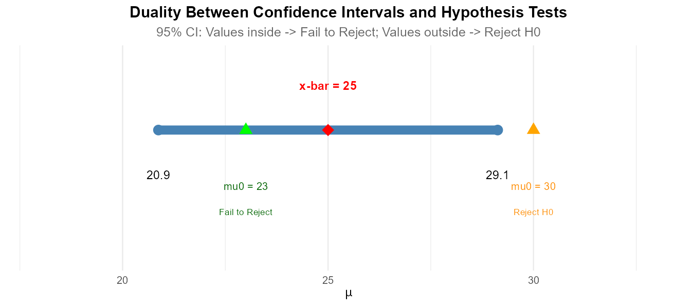
Fig. 10.28 Values inside the CI lead to non-rejection; values outside lead to rejection.

For a two-sided hypothesis test and confidence interval with matching confidence/significance levels (C + α = 1):

• If μ₀ is inside the CI → Fail to reject H₀

• If μ₀ is outside the CI → Reject H₀

This works because both procedures use the same information and criteria. The CI contains all values of μ that would not be rejected by the corresponding test.

---

Exercise 8: Duality - From Hypothesis Test to CI

A researcher conducts a two-sided t-test at α = 0.05 with:

• n = 25

• \(\bar{x} = 48.2\)

• s = 6.5

• μ₀ = 45

The test yields t_TS = 2.462 and p-value = 0.0213, leading to rejection of H₀.

1. Construct the corresponding 95% confidence interval.

2. Verify that μ₀ = 45 is outside this CI.

3. What would be the result of testing H₀: μ = 47 at α = 0.05?

Solution

Part (a): 95% Confidence Interval

df = 25 - 1 = 24

\(t_{0.025, 24} = 2.064\)

\[SE = \frac{s}{\sqrt{n}} = \frac{6.5}{\sqrt{25}} = 1.3\]

\[CI: \bar{x} \pm t_{0.025, 24} \times SE = 48.2 \pm 2.064 \times 1.3\]

\[= 48.2 \pm 2.68 = (45.52, 50.88)\]

Part (b): Verification

μ₀ = 45 is outside the CI (45.52, 50.88). ✓

This is consistent with rejecting H₀: μ = 45 at α = 0.05.

Part (c): Testing H₀: μ = 47

μ₀ = 47 is inside the CI (45.52, 50.88).

By duality: Fail to reject H₀ at α = 0.05.

R verification:

xbar <- 48.2; s <- 6.5; n <- 25
SE <- s / sqrt(n)  # 1.3
t_crit <- qt(0.025, df = 24, lower.tail = FALSE)  # 2.064
c(xbar - t_crit * SE, xbar + t_crit * SE)  # (45.52, 50.88)

---

Exercise 9: Using t.test() in R

A quality control engineer measures the tensile strength (in MPa) of 10 steel specimens:

425, 438, 412, 445, 428, 433, 419, 441, 436, 423

1. Calculate \(\bar{x}\) and s from this data.

2. Use R’s t.test() function to test H₀: μ = 420 vs Hₐ: μ ≠ 420 at α = 0.05.

3. Interpret the output, including the t-statistic, df, p-value, and CI.

4. What is your conclusion about the mean tensile strength?

Solution

Part (a): Summary Statistics

strength <- c(425, 438, 412, 445, 428, 433, 419, 441, 436, 423)
mean(strength)  # 430
sd(strength)    # 10.42

\(\bar{x} = 430\) MPa, s = 10.42 MPa

Part (b): t.test() Output

t.test(strength, mu = 420, alternative = "two.sided", conf.level = 0.95)

# Output:
# One Sample t-test
#
# data:  strength
# t = 3.0336, df = 9, p-value = 0.01422
# alternative hypothesis: true mean is not equal to 420
# 95 percent confidence interval:
#  422.5441 437.4559
# sample estimates:
# mean of x
#       430

Part (c): Interpretation

• t-statistic: t = 3.034

• Degrees of freedom: df = 9

• P-value: 0.0142

• 95% CI: (422.54, 437.46) MPa

The t-statistic of 3.034 indicates the sample mean is about 3 standard errors above μ₀ = 420.

The p-value of 0.0142 is less than α = 0.05.

The CI does not contain μ₀ = 420, consistent with rejection.

Part (d): Conclusion

The data does give support (p-value = 0.014) to the claim that the mean tensile strength differs from 420 MPa. The 95% CI suggests the true mean is between 422.5 and 437.5 MPa, indicating the steel may be slightly stronger than the 420 MPa specification.

---

Exercise 10: Application with Raw Data

A cognitive psychologist measures reaction times (in milliseconds) for 20 participants in a visual recognition task:

245, 238, 252, 241, 259, 247, 236, 255, 243, 249,
251, 240, 258, 244, 237, 253, 246, 250, 242, 248

The standard reaction time for this task is believed to be 250 ms. Test whether this sample suggests a different mean reaction time at α = 0.05.

1. State the hypotheses.

2. Calculate summary statistics.

3. Perform the t-test manually (calculate t_TS and p-value).

4. Verify using R’s t.test() function.

5. Construct the 95% CI and verify duality.

6. State your conclusion in context.

Solution

Part (a): Hypotheses

Let μ = true mean reaction time (ms).

\[H_0: \mu = 250 \quad \text{vs} \quad H_a: \mu \neq 250\]

Part (b): Summary Statistics

times <- c(245, 238, 252, 241, 259, 247, 236, 255, 243, 249,
           251, 240, 258, 244, 237, 253, 246, 250, 242, 248)
n <- length(times)    # 20
xbar <- mean(times)   # 246.7
s <- sd(times)        # 6.729

n = 20, \(\bar{x}\) = 246.7 ms, s = 6.73 ms

Part (c): Manual T-test

\[t_{TS} = \frac{246.7 - 250}{6.729 / \sqrt{20}} = \frac{-3.3}{1.505} = -2.193\]

df = 19

P-value (two-tailed):

\[p\text{-value} = 2 \times P(T_{19} > 2.193) = 0.0409\]

Part (d): R Verification

t.test(times, mu = 250)

# t = -2.1933, df = 19, p-value = 0.04094
# 95% CI: (243.5502, 249.8498)

Part (e): 95% CI and Duality

95% CI: (243.55, 249.85) ms

μ₀ = 250 is outside this CI (just barely).

By duality, this is consistent with rejecting H₀ at α = 0.05. ✓

Part (f): Conclusion

The data does give support (p-value = 0.041) to the claim that the mean reaction time for this task differs from the standard of 250 ms. The sample suggests participants responded slightly faster, with a mean around 246.7 ms. However, note that the p-value is close to 0.05, so this is a relatively weak rejection.

---

10.3.6. Additional Practice Problems

True/False Questions (1 point each)

1. The t-distribution is used when σ is unknown and must be estimated.

   Ⓣ or Ⓕ

2. As df increases, the t-distribution approaches the standard normal distribution.

   Ⓣ or Ⓕ

3. For a given test statistic value, the p-value from a t-test is smaller than from a z-test.

   Ⓣ or Ⓕ

4. Degrees of freedom for a one-sample t-test equals n.

   Ⓣ or Ⓕ

5. If μ₀ is inside a 95% CI, we would reject H₀ at α = 0.05.

   Ⓣ or Ⓕ

6. The t.test() function in R can perform both one-sided and two-sided tests.

   Ⓣ or Ⓕ

Multiple Choice Questions (2 points each)

7. For n = 20 and α = 0.05 (two-tailed), the t-critical value is:

   Ⓐ t₀.₀₅,₂₀

   Ⓑ t₀.₀₂₅,₂₀

   Ⓒ t₀.₀₂₅,₁₉

   Ⓓ t₀.₀₅,₁₉

8. If \(\bar{x} = 52\), μ₀ = 50, s = 8, n = 16, then t_TS equals:

   Ⓐ 0.25

   Ⓑ 1.00

   Ⓒ 2.00

   Ⓓ 4.00

9. A 90% CI is (45, 55). Testing H₀: μ = 58 at α = 0.10 leads to:

   Ⓐ Reject H₀

   Ⓑ Fail to reject H₀

   Ⓒ Cannot determine without more information

   Ⓓ Accept H₀

10. The t-test is more conservative than the z-test because:

    Ⓐ t-critical values are smaller

    Ⓑ t-critical values are larger (for finite df)

    Ⓒ t-tests use larger samples

    Ⓓ t-tests have smaller p-values

11. For t_TS = 2.5 with df = 10 (upper-tailed), the p-value is calculated as:

    Ⓐ pt(2.5, 10)

    Ⓑ pt(2.5, 10, lower.tail = FALSE)

    Ⓒ 2 * pt(2.5, 10, lower.tail = FALSE)

    Ⓓ 1 - pt(2.5, 10)

12. Which correctly pairs a CI type with a hypothesis test type for duality?

    Ⓐ 95% CI with α = 0.10 two-tailed test

    Ⓑ 95% CI with α = 0.05 two-tailed test

    Ⓒ 95% LCB with α = 0.05 two-tailed test

    Ⓓ 90% CI with α = 0.05 two-tailed test

Answers to Practice Problems

True/False Answers:

1. True — When σ is unknown, we use s and the t-distribution.

2. True — As df → ∞, t → z (standard normal).

3. False — T-distribution has heavier tails, so p-values are larger.

4. False — df = n - 1 for one-sample t-test.

5. False — If μ₀ is inside the CI, we fail to reject H₀.

6. True — Use alternative = "less" or "greater" for one-sided.

Multiple Choice Answers:

7. Ⓒ — For n = 20: df = 19, and two-tailed uses α/2 = 0.025.

8. Ⓑ — t_TS = (52 - 50)/(8/√16) = 2/2 = 1.00.

9. Ⓐ — 58 is outside (45, 55), so reject H₀ by duality.

10. Ⓑ — Larger critical values make rejection harder (more conservative).

11. Ⓑ — Upper-tailed: p-value = P(T > t_TS) = pt(t_ts, df, lower.tail = FALSE).

12. Ⓑ — Duality requires C + α = 1, so 95% CI pairs with α = 0.05.