Slides 📊

12.3. ANOVA F-Test and Its Relationship to Two-Sample t-Tests

We have developed the theoretical foundation for ANOVA by decomposing total variability into between-group and within-group components. Now we are ready to construct the hypothesis test that will tell us whether observed differences in sample means are statistically significant.

Road Map 🧭

Understand why the \(F\)-test statistic serves as an indicator of differences among population means.
Describe the properties of the \(F\) distributions.
Construct a complete ANOVA table and perform an ANOVA \(F\)-test using the four-step framework.
Recognize the connections between ANOVA and independent two-sample inference.

12.3.1. Building the Test Statistic

Recall the goal of the ANOVA hypothesis test: we would like to compare the variabilities within and between groups, and reject the null hypothesis that all means are equal if the between-group variability is significantly larger.

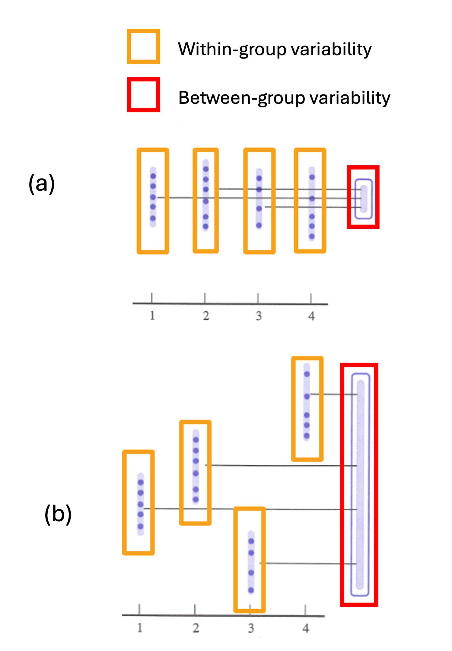
Comparison of within-group and between-group variation — Fig. 12.14 Within-group vs between-group variability

To formalize this comparison, we use the ratio between MSA and MSE.

\[\frac{\text{Between-group variability}}{\text{Within-group variability}} = \frac{\text{MSA}}{\text{MSE}}\]

When \(H_0\) is true, both MSA and MSE estimate \(\sigma^2\), so their observed ratio tends to be close to 1. When \(H_0\) is false, however, MSA estimates something larger, making it more likely for the ratio to take a value significantly larger than 1.

Under the null hypothesis, the distribution of the ratio belongs to the family of \(F\)-distributions. For this reason, the ratio is called the \(F\)-test statistic, or \(F_{TS}\). To complete the hypothesis testing construction, we next review the main properties of \(F\)-distributed random variables.

12.3.2. The \(F\)-Distribution

\(F\)-distributions are parameterized by two degrees of freedom: \(df_1\) and \(df_2\). When a ramdom variable \(X\) follows an \(F\)-distribution, we write:

\[X \sim F(df_1, df_2).\]

\(F\)-distributions are always supported on \([0, \infty)\) and are right-skewed regardless of the parameter values. As the two degrees of freedom grow,

the skewness weakens (see the yellow curve in Fig. 12.15),
the expected value quickly approaches 1, and
the variance decreases.

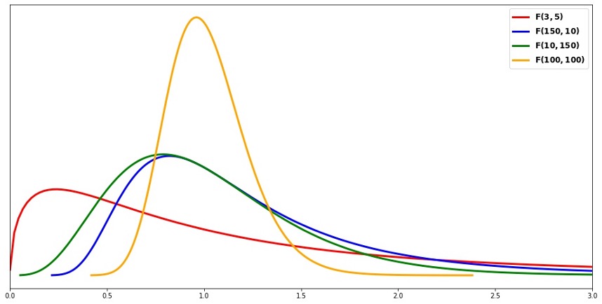
F-distributions with different sets of parameter values — Fig. 12.15 \(F\)-distribution with different sets of parameter values

Let us now discuss the specific \(F\) distribution of the ANOVA test statistic. Under the null hypothesis,

\[F_{TS} \sim F(df_A = k-1, df_E = n-k),\]

where \(k\) represents the number of groups and \(n\) the total sample size.

Drawing connections with the general properties of \(F\)-distributions,

\(F_{TS}\) will always yield a non-negative outcome since it is a ratio of two non-negative random variables. This agrees with the support of its null distribution.
As the total sample size \(n\) grows, the expected value of \(F_{TS}\) grows closer to 1 and its spread becomes narrower arround the mean.

The \(p\)-Value for ANOVA

Regardless of the analysis method, a \(p\)-value always represents the probability of obtaining a result more inconsistent with the null hypothesis than the one observed. In ANOVA, such inconsistency corresponds to a greater observed \(F\)-test statistic. Therefore,

\[\text{p-value} = P(F_{k-1,n-k} \geq f_{ts}),\]

where \(F_{k-1,n-k}\) is a random variable following an \(F\) distribution with \((df_1,df_2)=(k-1, n-k)\), and \(f_{TS}\) is the observed \(F\)-test statistic. On R, the \(p\)-value can be obtained using the pf function:

pvalue <- pf(f_ts, df1=k-1, df2=n-k, lower.tail=FALSE)

The Complete ANOVA Table

We are now fully equipped to construct the complete ANOVA table that we left partially filled in Chapter 12.2. The entries marked with ⅹ are typically left blank.

Source	df	SS	MS	\((f_{TS})\)	\(p\)-value
Factor A	\(k-1\)	\(\sum_{i=1}^k n_i(\bar{x}_{i \cdot} - \bar{x}_{\cdot \cdot})^2\)	\(\frac{\text{SSA}}{k-1}\)	\(\frac{MSA}{MSE}\)	\(P(F_{k-1,n-k} \geq f_{ts})\)
Error	\(n-k\)	\(\sum_{i=1}^k \sum_{j=1}^{n_i}(x_{ij} - \bar{x}_{i \cdot})^2\)	\(\frac{\text{SSE}}{n-k}\)	ⅹ	ⅹ
Total	\(n-1\)	\(\sum_{i=1}^k \sum_{j=1}^{n_i}(x_{ij} - \bar{x}_{\cdot \cdot})^2\)	ⅹ	ⅹ	ⅹ

Example 💡: The Complete ANOVA Table for the Coffeehouse Study

For the coffeehouse study, complete the remaining entries of the ANOVA table.

Table 12.3 Complete ANOVA Table
Source	df	SS	MS	\(f_{TS}\)	\(p\)-value
Factor A	4	8834	2208.4	22.14	\(4.4 \times 10^{-15}\)
Error	195	19451	99.8
Total	199	28285

We only need to fill the two entries corresponding to the observed \(f_{TS}\) and the \(p\)-value.

(1) First,

\[f_{TS} = \frac{MSA}{MSE} = \frac{2208.4}{99.8} = 22.14\]

Recall that under the null hypothesis and a total sample size as large as \(n=200\), the \(F\)-test statistic is distributed sharply around 1. The observed value of 22.10 already gives a strong sign of inconsistency with the null hypothesis.

(2) Let us continue to computing the \(p\)-value and check if our prediction is confirmed:

\[\text{p-value} = P(F_{4,195} \geq 22.10) = 4.89 \times 10^{-15}\]

As expected, the \(p\)-value is very small.

We are now ready to organize the ANOVA hypothesis test into a full four-step framework.

12.3.3. The Four Steps of ANOVA Hypothesis Testing

Step 1: Define Parameters

Define the population mean \(\mu_i\), for each \(i \in \{1, \cdots, k\}\). The definition should clearly describe the populations of interest and connect each \(\mu_i\) to a specific population.

Step 2: State the Hypotheses

\[\begin{split}&H_0: \mu_1 = \mu_2 = \cdots = \mu_k \\ &H_a: \mu_i \neq \mu_j \text{ for some } i \neq j\end{split}\]

The alternative hypothesis can be written in several equivalent ways:

\(H_a:\) At least one \(\mu_i\) is different from the rest
\(H_a:\) Not all population means are equal
\(H_a:\) At least one \(\mu_i\) differs from the others

Step 3-1: Check Assumptions

Before proceeding, we must verify that the ANOVA assumptions are reasonable. See Section 12.1.3 for a complete walkthrough of graphical verification. In addition, we must confirm numerically that the equal variance assumption is reasonable by showing:

\[\frac{\max(s_{1\cdot}, s_{2\cdot}, \ldots, s_{k\cdot})}{\min(s_{1\cdot}, s_{2\cdot}, \ldots, s_{k\cdot})} \leq 2.\]

Step 3-2: Calculate the Test Statistic, Degrees of Freedom, and \(p\)-Value

In this step, it is often helpful to first construct the full ANOVA table.

Use the computed MSA and MSE for the observed test statistic, \(f_{TS}\):

\[f_{TS} = \frac{\text{MSA}}{\text{MSE}}\]
State the degrees of freedom:
- \(df_A = k - 1\)
- \(df_E = n - k\)
Compute the \(p\)-value, \(P(F_{df_A, df_E} \geq f_{TS})\):

pf(f_ts, df1 = k-1, df2 = n-k, lower.tail = FALSE)

Step 4: Make Decision and State Conclusion

Decision rule stays unchanged:

If \(p\)-value \(\leq \alpha\), reject \(H_0\).
If \(p\)-value \(> \alpha\), fail to reject \(H_0\).

Conclusion template:

“The data [does/does not] give [weak/moderate/strong] support (p-value = [value]) to the claim that [statement of \(H_a\) in context].”

Performing ANOVA When Complete Data is Available

Suppose the complete dataset can be organized into a data.frame with two columns:

The column response_variable lists responses measurements for all groups.
The column factor_variable lists the group labels for each entry of response_variable in a matching order.

Then, the R function aov() can be used to run all ANOVA computations from scratch:

fit <- aov(response_variable ~ factor_variable, data = dataframe)

# output
summary(fit)

What Happens If \(H_0\) Is Rejected?

When ANOVA indicates that “at least one mean differs from the others,” it naturally raises the next question: “Which specific groups are different?” This brings us to multiple comparison procedures, explored in the next section. These methods allow specific pairwise comparisons while controlling the overall error rate.

For now, it’s important to understand that ANOVA serves as a gatekeeper test, screening data sets that require pairwise comparisons from those that do not.

Example💡: Complete ANOVA Testing for the Coffeehouse Data ☕️

Perform a hypothesis test at \(\alpha = 0.01\) to determine if the five coffeehouses around campus attract customers of different average ages.

📊 Download the coffeehouse dataset (CSV)

Table 12.4 Sample Statistics
Sample (Levels of Factor Variable)	Sample Size	Mean	Variance
Population 1	\(n_1 = 39\)	\(\bar{x}_{1.} = 39.13\)	\(s_1^2 = 62.43\)
Population 2	\(n_2 = 38\)	\(\bar{x}_{2.} = 46.66\)	\(s_2^2 = 168.34\)
Population 3	\(n_3 = 42\)	\(\bar{x}_{3.} = 40.50\)	\(s_3^2 = 119.62\)
Population 4	\(n_4 = 38\)	\(\bar{x}_{4.} = 26.42\)	\(s_4^2 = 48.90\)
Population 5	\(n_5 = 43\)	\(\bar{x}_{5.} = 34.07\)	\(s_5^2 = 98.50\)
Combined	\(n = 200\)	\(\bar{x}_{..} = 37.35\)	\(s^2 = 142.14\)

Step 1: Define the Parameters

Let \(\mu_{1}, \mu_{2}, \mu_{3}, \mu_{4}, \mu_{5}\) represent the true mean customer age at coffeehouses 1, 2, 3, 4, and 5, respectively.

Step 2: State the Hypotheses

\[\begin{split}&H_0: \mu_{1} = \mu_{2} = \mu_{3} = \mu_{4} = \mu_{5}\\ &H_a: \mu_{i} \neq \mu_{j} \text{ for some } i \neq j\end{split}\]

Step 3-1: Check Assumptions

This step should include all the following elements:

Graphical check for any serious deviations from normality in individual samples
Graphical check for any signs of violation of the equal variance assumption
Using the numerical method to confirm that the sample variances (standard deviations) are within similar ranges:

\[\frac{\max{s_i}}{\min{s_i}} = \frac{\sqrt{168.34}}{\sqrt{48.90}} = 1.855 < 2 \checkmark\]

Refer to the last example of Chapter 12.1.

Step 3-2: Calculate the Test Statistic, Degrees of Freedom, and p-Value

Table 12.5 Complete ANOVA Table
Source	df	SS	MS	\(f_{TS}\)	\(p\)-value
Factor A	4	8834	2208.4	22.14	\(4.4 \times 10^{-15}\)
Error	195	19451	99.8
Total	199	28285

Test statistic: \(f_{TS} = 22.14\)
Degrees of freedom for the null distribution: \(df_A = 4\), \(df_E = 195\)
\(p\)-value \(= 4.4 \times 10^{-15}\)

Step 4: Decision and Conclusion

Since p-value = \(4.4 \times 10^{-15} < 0.01 = \alpha\), we reject \(H_0\).

The data gives strong support (p-value = \(4.4 \times 10^{-15}\)) to the claim that at least one of the coffeehouses around campus differs in the mean age of customers from the rest.

12.3.4. The Connection Between F-Tests and t-Tests

It is possible to view one-way ANOVA as a generalization of independent two-sample analysis under certain conditions. Specifically, one-way ANOVA with \(k=2\) is equivalent to a two-tailed independent two-sample hypothesis test with \(\Delta_0=0\) and the equal variance assumption.

We show this special relationship by demonstrating that the \(F\)-test statistic for ANOVA is equal to the square of the \(t\)-test statistic for the two-sammple comparison. In turn, we also show that the \(p\)-values computed from these two statistics are identical.

Connection Between the Test Statistics

When \(k=2\), the ANOVA \(F\)-test statistic is:

\[F_{TS} = \frac{\text{MSA}}{\text{MSE}} = \frac{n_1(\bar{X}_{1\cdot} - \bar{X}_{\cdot \cdot})^2 + n_2(\bar{X}_{2\cdot} - \bar{X}_{\cdot \cdot})^2}{\frac{(n_1-1)S_{1\cdot}^2 + (n_2-1)S_{2\cdot}^2}{n_1 + n_2 - 2}}.\]

Through algebraic manipulation (which involves expressing the overall mean \(\bar{X}_{\cdot \cdot}\) as a weighted average of the group means), this simplifies to:

\[F_{TS} = \frac{(\bar{X}_{1\cdot} - \bar{X}_{2\cdot})^2}{S_p^2\left(\frac{1}{n_1} + \frac{1}{n_2}\right)}.\]

Recall the \(t\)-test statistic for independent two-sample comparison with the pooled variance estimator:

\[T_{TS} = \frac{(\bar{X}_1 - \bar{X}_2) - \Delta_0}{S_p\sqrt{\frac{1}{n_1} + \frac{1}{n_2}}}.\]

By setting \(\Delta_0 = 0\) and squaring \(T_{TS}\), we recover \(F_{TS}\).

Equivalence of the \(p\)-Values

Using the connection between the two test statistics, the ANOVA \(p\)-value satisfies:

\[P(F_{1, n-2} > f_{TS}) = P(T_{n-2}^2 > t^2_{TS}) = P(|T_{n-2}| > |t_{TS}|) = 2P(T_{n-2} > |t_{TS}|)\]

The final probability statement is, in fact, the \(p\)-value for the two-sided \(t\)-test. That is, the \(p\)-value computed through one-way ANOVA is identical to the \(p\)-value computed from a two-sided test for difference between two means.

It follows that the decision to reject or fail to reject the null hypothesis is also identical—essentially, the two tests are the same procedure in difference forms.

Summary

In summary, ANOVA with \(k=2\) is equivalent to an independent two-sample analysis with the equal variance assumption and a null value of zero. Between the two options, then, what should we choose? The decision depends on whether you value the flexibility of the two-sample analysis or the generalizability of ANOVA.

Comparison of Independent Two-Sample \(t\)-Test and ANOVA
Feature	Indepdent Two-Sample \(t\)-Test	One-Way ANOVA
Variance Assumption	Can assume equal or unequal variances among groups	Assumes equal variances
Hypothesis Type	Any direction can be chosen	Two-sided only
Null Value \(\Delta_0\)	Can by any value	Limited to \(\Delta_0 = 0\)
Number of Groups	Exactly 2 groups	2 or more groups

12.3.5. Bringing It All Together

Key Takeaways 📝

The F-test statistic \(\frac{\text{MSA}}{\text{MSE}}\) compares between-group to within-group variability, with large values providing evidence against \(H_0\).
The F-distribution is right-skewed, non-negative, and with mean approximately 1.s Its shape is controlled by two degrees of freedom. Under the null hypothesis, the \(F\)-test statistic follows an \(F\) distribution with \(df_1=k-1\) and \(df_2=n-k\).
The ANOVA table organizes all components of ANOVA, including the \(F\)-test statistic and the \(p\)-value.
The complete ANOVA hypothesis testing follows the standard four-step framework.
ANOVA \(F\)-tests with \(k=2\) are equivalent to certain two-sample \(t\)-tests.
ANOVA serves as a gatekeeper test that determines whether any group differences exist before investigating specific pairwise comparisons.

12.3.6. Exercises

Exercise 1: Properties of the F-Distribution

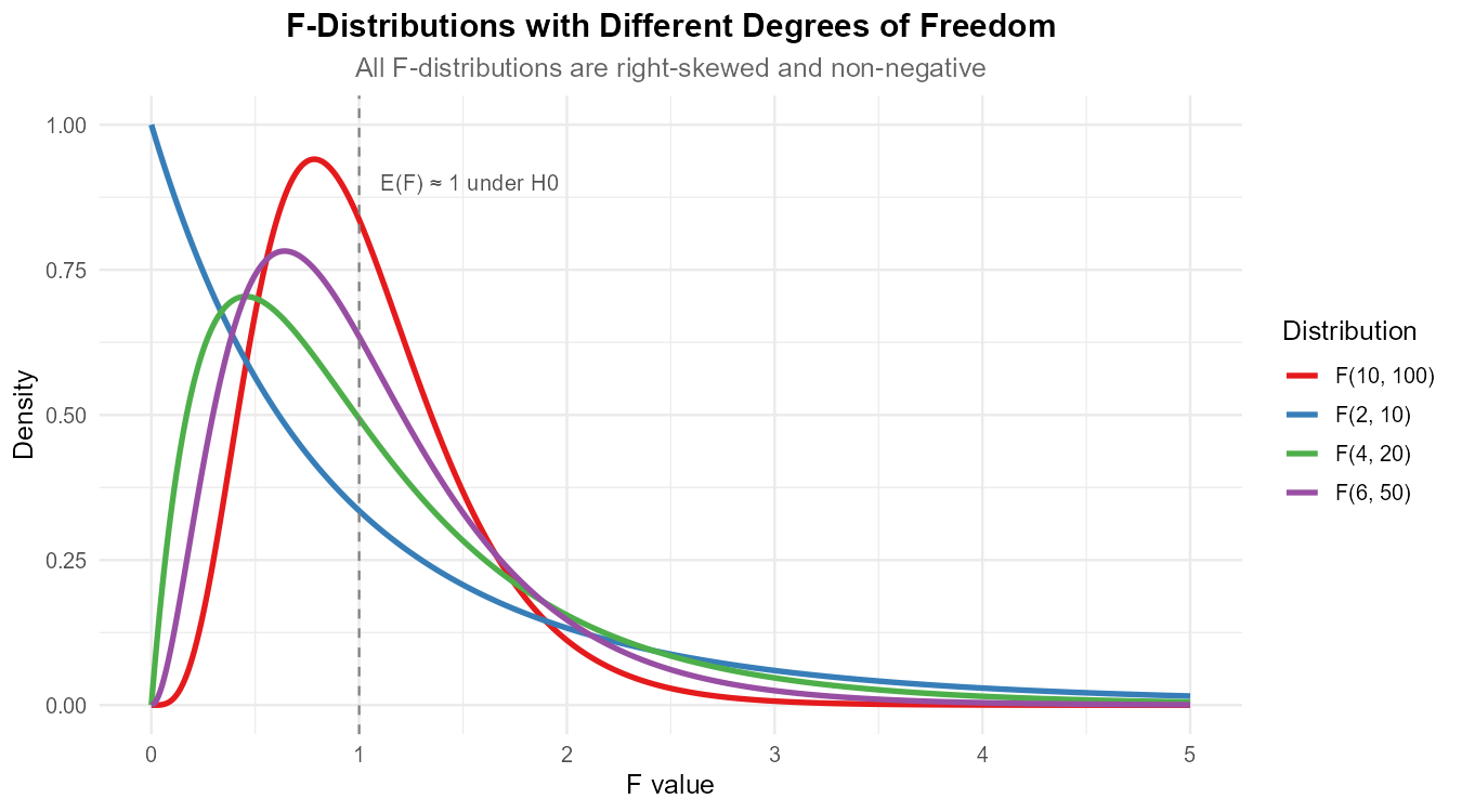
F-distributions with different degrees of freedom — Fig. 12.16 **Figure 1**: F-distributions with various degrees of freedom parameters.

Refer to Figure 1 showing F-distributions with different parameter values.

What are the two parameters that define an F-distribution? What do they represent in ANOVA?
What is the support (range of possible values) of an F-distribution? Why does this make sense for the F-statistic?
As both degrees of freedom increase, what happens to the shape of the F-distribution?
Under H₀, what value should the F-statistic be centered near? Explain.
Why are F-tests always right-tailed (one-sided) rather than two-tailed?

Exercise 2: Computing the F-Test Statistic

Using the blood glucose monitoring device data from Exercise 8 of Section 12.2, the partial ANOVA table is:

Source	df	SS	MS
Device	2	6.93	3.47
Error	12	2.62	0.22
Total	14	9.55

Calculate the F-test statistic.
Interpret the F-statistic value. What does it tell us about the ratio of between-group to within-group variability?
Using R’s pf() function, calculate the p-value. Show the R code.
At α = 0.05, what is your decision regarding H₀?

Exercise 3: Complete Four-Step ANOVA Hypothesis Test

A software engineer compares the execution time (in milliseconds) of four different sorting algorithms on datasets of size n = 10,000. Each algorithm is run 15 times. Summary results:

Algorithm	n	Mean (ms)	SD (ms)
QuickSort	15	45.2	5.8
MergeSort	15	52.1	6.2
HeapSort	15	58.7	5.5
IntroSort	15	47.3	6.0

Conduct a complete ANOVA hypothesis test at α = 0.01.

Solution

Step 1: Define the parameters

Let \(\mu_i\) = true mean execution time (ms) for algorithm i, where:

\(\mu_1\) = mean for QuickSort
\(\mu_2\) = mean for MergeSort
\(\mu_3\) = mean for HeapSort
\(\mu_4\) = mean for IntroSort

Step 2: State the hypotheses

\[\begin{split}&H_0: \mu_1 = \mu_2 = \mu_3 = \mu_4\\ &H_a: \text{At least one } \mu_i \text{ is different from the others}\end{split}\]

In words: H₀ states all algorithms have equal mean execution times. Hₐ states at least one algorithm has a different mean execution time.

Step 3: Check assumptions and calculate test statistic

Assumption checks:

Independence: Assumed satisfied by the experimental design (separate algorithm runs).
Equal variances (can verify from summary statistics):

\[\frac{\max(s_i)}{\min(s_i)} = \frac{6.2}{5.5} = 1.13 \leq 2 \quad \checkmark\]

Normality: With only summary statistics provided, we cannot create visual diagnostics. However, with n = 15 per group (total n = 60), ANOVA is reasonably robust to moderate departures from normality. Assume normality is approximately satisfied based on the nature of execution time measurements.

Calculate grand mean:

\[\bar{x}_{..} = \frac{15(45.2) + 15(52.1) + 15(58.7) + 15(47.3)}{60} = \frac{3049.5}{60} = 50.825\]

Calculate SSA:

\[\text{SSA} = 15[(45.2-50.825)^2 + (52.1-50.825)^2 + (58.7-50.825)^2 + (47.3-50.825)^2]\]

\[= 15[31.64 + 1.63 + 62.00 + 12.43] = 15(107.70) = 1615.5\]

Calculate SSE:

\[\text{SSE} = 14(5.8^2) + 14(6.2^2) + 14(5.5^2) + 14(6.0^2)\]

\[= 14(33.64 + 38.44 + 30.25 + 36.00) = 14(138.33) = 1936.62\]

Calculate degrees of freedom:

\(df_A = k - 1 = 3\)
\(df_E = n - k = 56\)

Calculate mean squares:

\[\text{MSA} = \frac{1615.5}{3} = 538.5, \quad \text{MSE} = \frac{1936.62}{56} = 34.58\]

Calculate F-statistic:

\[F_{TS} = \frac{538.5}{34.58} = 15.57\]

Calculate p-value:

\[\text{p-value} = P(F_{3,56} \geq 15.57) = 1.75 \times 10^{-7}\]

Complete ANOVA Table:

Source	df	SS	MS	F	p-value
Algorithm	3	1615.5	538.5	15.57	1.75×10⁻⁷
Error	56	1936.6	34.58
Total	59	3552.1

Step 4: Decision and Conclusion

Since p-value = 1.75 × 10⁻⁷ < 0.01 = α, we reject H₀.

Conclusion: At the 0.01 significance level, there is sufficient evidence to conclude that at least one sorting algorithm has a different mean execution time than the others (p < 0.001). Further analysis (multiple comparisons) is needed to determine which specific algorithms differ.

R verification:

n <- c(15, 15, 15, 15)
xbar <- c(45.2, 52.1, 58.7, 47.3)
s <- c(5.8, 6.2, 5.5, 6.0)

grand_mean <- sum(n * xbar) / sum(n)  # 50.825
SSA <- sum(n * (xbar - grand_mean)^2)  # 1615.5
SSE <- sum((n - 1) * s^2)  # 1936.62

df_A <- 3; df_E <- 56
MSA <- SSA / df_A  # 538.5
MSE <- SSE / df_E  # 34.58

F_ts <- MSA / MSE  # 15.57
p_value <- pf(F_ts, df_A, df_E, lower.tail = FALSE)  # 2.07e-7

Exercise 4: ANOVA Table Completion

Complete the missing entries in each ANOVA table.

(a) Manufacturing study with 5 production methods:

Source	df	SS	MS	F	p-value
Method	___	840	___	___	___
Error	45	___	30
Total	___	2190

(b) Clinical trial with 3 drug dosages (total n = 75):

Source	df	SS	MS	F	p-value
Dosage	___	___	156.2	4.87	___
Error	___	___	___
Total	___	2620.4

Solution

(a) Manufacturing study:

Step 1: Degrees of freedom

df_A = k - 1 = 5 - 1 = 4
df_E = 45 (given)
df_T = df_A + df_E = 4 + 45 = 49

Step 2: Sums of Squares

SSE = MSE × df_E = 30 × 45 = 1350
SSA = 840 (given)
Check: SSA + SSE = 840 + 1350 = 2190 = SST ✓

Step 3: MSA and F

MSA = SSA/df_A = 840/4 = 210
F = MSA/MSE = 210/30 = 7.0

Step 4: p-value

p-value = P(F_{4,45} ≥ 7.0) = 0.00018

Source	df	SS	MS	F	p-value
Method	4	840	210	7.0	0.00018
Error	45	1350	30
Total	49	2190

(b) Clinical trial:

Step 1: Degrees of freedom

k = 3 dosages → df_A = 2
n = 75 → df_T = 75 - 1 = 74
df_E = df_T - df_A = 74 - 2 = 72

Step 2: Mean squares

MSA = 156.2 (given)
F = MSA/MSE → MSE = MSA/F = 156.2/4.87 = 32.07

Step 3: Sums of Squares

SSA = MSA × df_A = 156.2 × 2 = 312.4
SSE = MSE × df_E = 32.07 × 72 = 2309.04
Check: 312.4 + 2309.0 ≈ 2621.4 ≈ 2620.4 (rounding) ✓

Step 4: p-value

p-value = P(F_{2,72} ≥ 4.87) = 0.0103

Source	df	SS	MS	F	p-value
Dosage	2	312.4	156.2	4.87	0.0103
Error	72	2308.0	32.06
Total	74	2620.4

R verification:

# Part (a)
pf(7.0, 4, 45, lower.tail = FALSE)  # 0.00018

# Part (b)
MSA <- 156.2
F_ts <- 4.87
MSE <- MSA / F_ts  # 32.07
pf(4.87, 2, 72, lower.tail = FALSE)  # 0.0104

Exercise 5: The F = t² Relationship

This exercise demonstrates that ANOVA with k = 2 is equivalent to a two-sided pooled two-sample t-test.

A researcher compares the yield (kg/plot) of two fertilizer types:

Fertilizer A: n₁ = 12, x̄₁ = 45.8, s₁ = 6.2
Fertilizer B: n₂ = 15, x̄₂ = 52.3, s₂ = 5.8

Conduct the comparison using a two-sample pooled t-test (H₀: μ₁ = μ₂ vs Hₐ: μ₁ ≠ μ₂). Report the t-statistic and p-value.
Conduct the comparison using one-way ANOVA. Report the F-statistic and p-value.
Verify that F = t².
Verify that the p-values are identical.
Under what conditions does this equivalence hold?

Exercise 6: Interpreting F-Values

For each scenario, interpret what the F-statistic value suggests and predict the likely outcome.

F = 0.85 with df₁ = 3 and df₂ = 40
F = 4.21 with df₁ = 4 and df₂ = 75
F = 12.56 with df₁ = 2 and df₂ = 27
F = 1.02 with df₁ = 5 and df₂ = 120

Exercise 7: Using R’s aov() Function with Complete Assumption Checking

A quality control engineer collects data on the fill volume (mL) of bottles from four production lines. The following R code creates and analyzes the data:

# Create the dataset
Line <- factor(rep(c("Line1", "Line2", "Line3", "Line4"), each = 10))
Volume <- c(
  # Line 1
  502.3, 498.7, 501.2, 499.8, 500.5, 503.1, 497.9, 501.8, 500.2, 499.5,
  # Line 2
  505.2, 504.8, 506.1, 503.9, 505.5, 504.2, 507.3, 505.8, 504.4, 506.8,
  # Line 3
  500.1, 499.3, 501.5, 498.7, 500.8, 499.2, 502.1, 500.4, 498.9, 501.3,
  # Line 4
  503.8, 502.9, 504.5, 501.7, 503.2, 505.1, 502.4, 504.8, 503.1, 504.5
)

fill_data <- data.frame(Line, Volume)

# Fit ANOVA model
fit <- aov(Volume ~ Line, data = fill_data)
summary(fit)

The output is:

             Df Sum Sq Mean Sq F value   Pr(>F)
Line         3  261.0   87.01   35.72 1.22e-10 ***
Residuals   36   87.7    2.44
---
Signif. codes:  0 '***' 0.001 '**' 0.01 '*' 0.05 '.' 0.1 ' ' 1

Before interpreting results, verify the ANOVA assumptions using appropriate visualizations. Show the R code for boxplots, faceted histograms, and faceted QQ-plots.
Interpret each column of the ANOVA output.
What are the null and alternative hypotheses being tested?
Based on the output, what is your conclusion at α = 0.05?
Estimate the common standard deviation σ.
What would be the next step in the analysis?

Solution

Part (a): Assumption checking

Before interpreting ANOVA results, we must verify the assumptions:

1. Equal Variance Check - Boxplots and SD Ratio:

library(ggplot2)

# Side-by-side boxplots
ggplot(fill_data, aes(x = Line, y = Volume, fill = Line)) +
  stat_boxplot(geom = "errorbar", width = 0.3) +
  geom_boxplot() +
  stat_summary(fun = mean, geom = "point", shape = 18,
               size = 3, color = "black") +
  ggtitle("Fill Volume by Production Line") +
  xlab("Production Line") +
  ylab("Fill Volume (mL)") +
  theme_minimal() +
  theme(legend.position = "none")

# Numerical SD ratio check
s <- tapply(fill_data$Volume, fill_data$Line, sd)
cat("Group SDs:", round(s, 3), "\n")
cat("SD ratio:", round(max(s)/min(s), 3), "\n")
# SD ratio = 1.47 (< 2) ✓ Equal variance assumption met

2. Normality Check - Faceted Histograms:

# Calculate group statistics
xbar <- tapply(fill_data$Volume, fill_data$Line, mean)
s <- tapply(fill_data$Volume, fill_data$Line, sd)

# Add normal density column
fill_data$normal.density <- mapply(function(vol, line) {
  dnorm(vol, mean = xbar[line], sd = s[line])
}, fill_data$Volume, fill_data$Line)

# Faceted histograms
ggplot(fill_data, aes(x = Volume)) +
  geom_histogram(aes(y = after_stat(density)),
                 bins = 6, fill = "grey", col = "black") +
  geom_density(col = "red", linewidth = 1) +
  geom_line(aes(y = normal.density), col = "blue", linewidth = 1) +
  facet_wrap(~ Line, ncol = 2) +
  ggtitle("Normality Check: Histograms by Line") +
  xlab("Fill Volume (mL)") +
  ylab("Density") +
  theme_minimal()

3. Normality Check - Faceted QQ-Plots:

ggplot(fill_data, aes(sample = Volume)) +
  stat_qq() +
  stat_qq_line(color = "red", linewidth = 1) +
  facet_wrap(~ Line, ncol = 2) +
  ggtitle("Normality Check: QQ-Plots by Line") +
  xlab("Theoretical Quantiles") +
  ylab("Sample Quantiles") +
  theme_minimal()

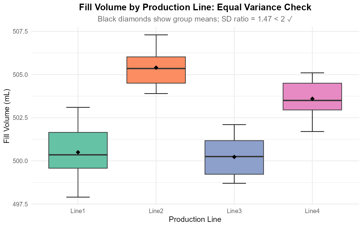
Fill volume boxplots by production line — Fig. 12.17 Side-by-side boxplots for equal variance assessment.

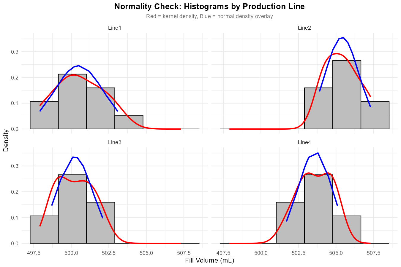
Fill volume histograms by production line — Fig. 12.18 Faceted histograms with kernel density (red) and normal overlay (blue).

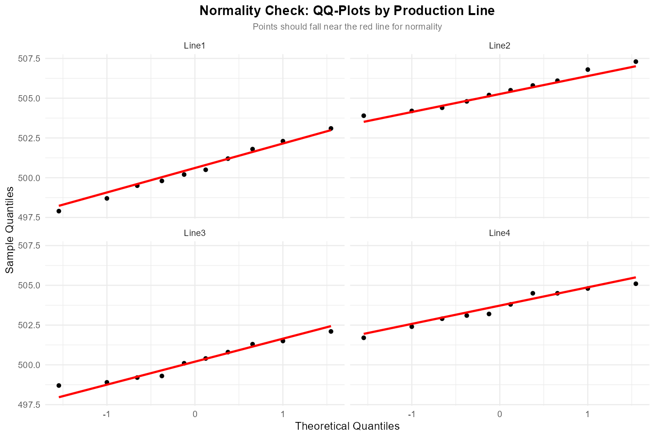
Fill volume QQ-plots by production line — Fig. 12.19 Faceted QQ-plots for normality assessment.

Assumption Summary:

Equal variances: SD ratio = 1.47 < 2 ✓ (boxplots show similar spread)
Normality: Histograms and QQ-plots show approximately normal distributions within each group ✓
Independence: Assumed from study design (separate production lines)

All assumptions are reasonably met; we can proceed with ANOVA interpretation.

Part (b): Column interpretation

Df: Degrees of freedom - Line (Factor): df_A = k - 1 = 4 - 1 = 3 - Residuals (Error): df_E = n - k = 40 - 4 = 36
Sum Sq: Sums of squares - SSA = 261.0 (between-group variability) - SSE = 87.7 (within-group variability)
Mean Sq: Mean squares - MSA = 261.0/3 = 87.01 - MSE = 87.7/36 = 2.44
F value: F-statistic = MSA/MSE = 87.01/2.44 = 35.72
Pr(>F): p-value = 1.22 × 10⁻¹⁰

Part (c): Hypotheses

H₀: μ₁ = μ₂ = μ₃ = μ₄ (all production lines have equal mean fill volumes)
Hₐ: At least one μᵢ is different (at least one line differs in mean fill volume)

Part (d): Conclusion at α = 0.05

Since p-value = 1.22 × 10⁻¹⁰ << 0.05 = α, we reject H₀.

Conclusion: At the 0.05 significance level, there is overwhelming evidence that at least one production line has a different mean fill volume than the others (p < 0.001). The very small p-value indicates extremely strong evidence against H₀.

Part (e): Estimate σ

\[\hat{\sigma} = \sqrt{\text{MSE}} = \sqrt{2.44} = 1.56 \text{ mL}\]

This represents the estimated within-line standard deviation of fill volumes.

Part (f): Next step

Since we rejected H₀, the next step is to perform multiple comparisons (post-hoc analysis) to identify which specific production lines differ from each other. We could use:

Tukey’s HSD (recommended for all pairwise comparisons)
Bonferroni correction

TukeyHSD(fit, conf.level = 0.95)

Exercise 8: When ANOVA Fails to Reject H₀

A researcher compares exam scores across three teaching methods and obtains:

F = 1.84
df₁ = 2, df₂ = 57
p-value = 0.168

State the conclusion at α = 0.05.
Does failing to reject H₀ prove that all population means are equal? Explain.
List three reasons why the test might fail to reject H₀ even if true differences exist.
What could the researcher do to increase the chance of detecting differences if they exist?

Exercise 9: Critical Value Approach

Instead of computing p-values, hypothesis tests can also be conducted using critical values.

For an ANOVA with k = 4 groups and n = 40 total observations at α = 0.05:

Determine the appropriate degrees of freedom.
Find the critical value F* such that P(F_{df₁, df₂} ≥ F*) = 0.05.
If the computed F-statistic is F = 3.12, what is the decision?
Compare this approach to using p-values. What are the advantages and disadvantages of each?

12.3.7. Additional Practice Problems

True/False Questions (1 point each)

If F = MSA/MSE = 2.5, it means the between-group variance is 2.5 times the within-group variance.

Ⓣ or Ⓕ
The p-value for an ANOVA F-test is calculated as P(F ≤ f_TS).

Ⓣ or Ⓕ
An F-statistic less than 1 always indicates that the null hypothesis is true.

Ⓣ or Ⓕ
For k = 2 groups, the ANOVA F-statistic equals the square of the pooled two-sample t-statistic.

Ⓣ or Ⓕ
The F-distribution is symmetric around its mean.

Ⓣ or Ⓕ
A very large F-statistic (e.g., F = 50) suggests strong evidence that at least one population mean differs from the others.

Ⓣ or Ⓕ

Multiple Choice Questions (2 points each)

Which R code correctly computes the p-value for an ANOVA F-test with F = 4.5, df₁ = 3, df₂ = 45?

Ⓐ pf(4.5, 3, 45)

Ⓑ pf(4.5, 3, 45, lower.tail = FALSE)

Ⓒ 1 - pf(4.5, 45, 3)

Ⓓ qf(4.5, 3, 45)
Under the null hypothesis, the expected value of the F-statistic is approximately:

Ⓐ 0

Ⓑ 1

Ⓒ k (number of groups)

Ⓓ n (total sample size)
Which of the following would NOT result in the F = t² relationship holding?

Ⓐ Using Welch’s t-test instead of pooled t-test

Ⓑ Having k = 2 groups

Ⓒ Testing H₀: μ₁ - μ₂ = 0

Ⓓ Using a two-sided alternative hypothesis
An ANOVA F-test yields p-value = 0.03. At α = 0.01, we:

Ⓐ Reject H₀ because 0.03 < 1

Ⓑ Reject H₀ because 0.03 < 0.05

Ⓒ Fail to reject H₀ because 0.03 > 0.01

Ⓓ Cannot determine without more information
The F-distribution with df₁ = 1 and df₂ = n-2 is related to which other distribution?

Ⓐ Normal distribution

Ⓑ Chi-square distribution

Ⓒ t-distribution squared

Ⓓ Exponential distribution