Slides 📊

12.1. Introduction to One-Way ANOVA

Many important research questions involve comparing two or more populations simultaneously. We now need a new approach that can handle the complexity of simultaneous comparisons while controlling the overall error rates.

Road Map 🧭

Identify the experimental conditions that call for the use of ANOVA.
Explain why a comparison of multiple means is called an Analysis of “Variance.”
Define the notations and formulate the hypotheses for ANOVA.
List the assumptions required for validity of ANOVA.

12.1.1. The Fundamental ANOVA Question

Many controlled experiments involve dividing subjects into two or more groups, applying a distinct treatment to each group, and then analyzing their quantitative responses to see if any systematic difference exists among the groups. See the example below for concrete scenarios.

Examples 💡: Experiments That Require Multiple Comparisons

Example 1: Bacterial Growth Study

A research group studies bacteria growth rates in different sugar solutions.

Factor variable: Type of sugar solution
Levels: Glucose, Sucrose, Fructose, Lactose (4 groups)
Quantitative response variable: Bacterial growth rate

Example 2: Gasoline Brand Efficiency

Researchers want to determine if five different gasoline brands affect automobile fuel efficiency.

Factor variable: Gasoline brand
Levels: Brand A, Brand B, Brand C, Brand D, Brand E (5 groups)
Quantitative response variable: Miles per gallon

The Research Question and Our Strategy

In all the examples above, the researchers aim to determine whether any difference exists among the true means of the response groups.

A naive approach to would be to perform two-sample comparisons for all possible pairs of levels. However, there are two critical drawbacks to this approach.

Let \(k\) be the number of levels. The total number of pairwise comparisons is \(k \choose 2\), which grows quickly with \(k\)—for example, \(10\) for \(k=5\) and \(45\) for \(k=10\).
When many inferences are performed simultaneously at significance level \(\alpha\), the probability of making at least one Type I error becomes substantially larger than \(\alpha\).

To avoid unncessary efforts and potential errors, we would like to first perform a single screening hypothesis test which determines whether any difference exists among the population means. Only when we reject the null hypothesis that all means are equal do we proceed to pairwise comparisons, taking special care to control the overall Type I error rate.

The preliminary screening test is called the Analysis of Variance, or ANOVA.

Why Analysis of “Variance”?

At first glance, it seems strange that a procedure designed to compare means is called an analysis of “variance.” This is because the perceived difference among means depend on the relative variances within and between groups. See Fig. 12.1 for a graphical illustration.

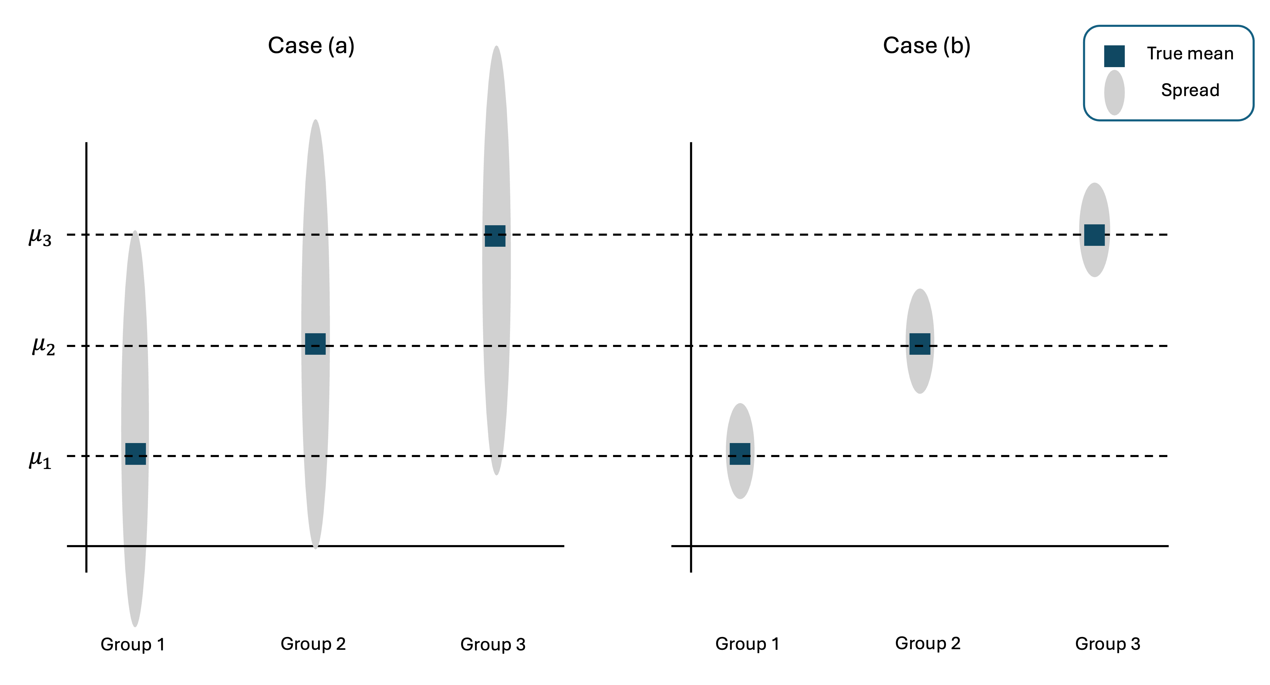
Graphical illustration of need for ANOVA — Fig. 12.1 Left: Distributions with large within-group variances; Right: Distributions with small within-group variances

Suppose we obtain samples from Case (a). Most likely, the data points will be spread over a wide range within each group. The within-group variability is wide enough to obscure the distinction created by the difference in central values.

On the other hand, samples from Case (b) will bunch closely arount their respective means, providing a stronger evidence that the true means are indeed distinct.

Note that the true means are identical in both cases—the absolute locations of the true means did not have a significant role in our visual analysis. Instead, the key difference arose from the relative size of the within-group spread in comparison with the spread of the true means.

If the within-group variation is comparable or larger than the between-group variation, we do not have enough evidence to reject the baseline belief that all means are equal.
If the within-group variation is smaller than the spread of the group means, there is a strong evidence that at least one true mean is different than the rest.

Why “One-Way”?

We use the term one-way ANOVA to indicate an experimental design in which groups are formed based on different levels of a single factor.

When analyzing the joint impact of two factors on a response, we use a two-way ANOVA. While the foundational ideas are the same as in one-way ANOVA, an additional feature must be considered—the interaction effect between the two factors, which may amplify or offset their respective main effects. ANOVA models involving more than two factors also exist.

In this course, we focus exclusively on one-way ANOVA.

12.1.2. Formalizing ANOVA

Notation

Suppose we have \(k\) different groups, where \(k \geq 2\).

ANOVA Notations for Group \(i\)
Group Index	\[i \in \{1, 2, \ldots, k\}\]
Observation Index	\[j \in \{1, 2, \ldots, n_i\}\]
Population Mean and Variance	\[\mu_i \text{ and } \sigma^2_i\]
Group Sample Size	\[n_i\]
Group Sample	\[X_{i1}, X_{i2}, \cdots, X_{in_i}\]
Group Sample Mean	\[\bar{X}_{i\cdot} = \frac{1}{n_i}\sum_{j=1}^{n_i} X_{ij}\]
Group Sample Variance	\[S_{i\cdot}^2 = \frac{1}{n_{i}-1}\sum_{j=1}^{n_i}(X_{ij} - \bar{X}_{i\cdot})^2\]
ANOVA Notation for Overall Summary
Overall Sample Size	\[n = n_1 + n_2 + \cdots + n_k\]
Overall Sample Mean	\[\bar{X}_{\cdot \cdot} = \frac{1}{n} \sum_{i=1}^{k} \sum_{j=1}^{n_i} X_{ij} = \frac{1}{n} \sum_{i=1}^{k} n_i \bar{X}_{i \cdot}\]

Each random variable in a sample is now indexed with double subscripts.

The first subscript \(i\) specifies the group to which the data point belongs.
The second subscript \(j\) indicates the observeration index within the group.

In addition, we use \(\cdot\) in the place of an index to indicate that a summary statistic is computed over all values of the corresponding index.

For example, the notation \(\bar{X}_{i\cdot}\) indiates that the statistic is computed using data points for all values of the second index, while keeping the group index fixed at \(i\).
Likewise, \(\bar{X}_{\cdot \cdot}\) means that data points for all indices are used to compute the summary.

Hypothesis Formulation

There is only one type of dual hypothesis for one-way ANOVA. The null hypothesis states that all true means are equal:

\(H_0: \mu_1 = \mu_2 = \mu_3 = \cdots = \mu_k.\)

The alternative hypothesis states that at least one population mean is different from the others. This can be expressed in several equivalent ways:

\(H_a:\) At least one \(\mu_i\) is different from the others.
\(H_a:\) Not all population means are equal.
\(H_a: \mu_i \neq \mu_j \text{ for some } i \neq j\)

Important Note About the Alternative

❌ It is incorrect to write the alternative hypothesis as

\[H_0: \mu_1 \neq \mu_2 \neq \mu_3 \neq \cdots \neq \mu_k.\]

The alternative hypothesis does not state that all means are different from each other. It only requires that at least one mean differs from the others. This could mean:

Only \(\mu_1\) differs from \(\mu_2 = \mu_3 = \mu_4\)
Two groups differ: \(\mu_1 = \mu_2 \neq \mu_3 = \mu_4\)
All groups differ: \(\mu_1 \neq \mu_2 \neq \mu_3 \neq \mu_4\)

Example 💡: Coffeehouse Demographics Study ☕️

A student reporter wants to study the demographics of coffeehouses around campus. Specifically, she’s interested in whether different coffeehouses attract customers of different ages. The reporter randomly selects 50 customers at each of five coffeehouses using a systematic sampling approach. Due to non-response, the final sample sizes vary slightly across coffeehouses but remain close to 50 per location.

Component Identification

Factor variable: Coffeehouse location (5 levels)
Response variable: Customer age (quantitative, measured in years)
Research question: Are there statistically significant differences between the average ages of customers at the different coffeehouses?

ANOVA Setup

Let \(\mu_i\) represent the true mean age of customers at Coffeehouse \(i\), for each \(i = 1, 2, \cdots , 5\). The hypotheses are:

\[\begin{split}&H_0: \mu_1 = \mu_2 = \mu_3 = \mu_4 = \mu_5 \\ &H_a: \mu_i \neq \mu_j \text{ for some } i \neq j\end{split}\]

Assumptions

Like all statistical procedures, ANOVA relies on certain assumptions for validity. These assumptions extend the familiar requirements from two-sample procedures to the multi-group setting.

Assumption 1: Independent Simple Random Samples

The observations in each of the \(k\) groups must form a simple random sample. That is, within each group \(i\), the observations \(X_{i1}, X_{i2}, \ldots, X_{in_i}\) must be independent and identically distributed.

Assumption 2: Independence Between Groups

Samples from different populations must be independent of each other.

Assumption 3: Normality of the Sample Means

Each population must either be normally distributed or have a large enough sample size for the CLT to hold, so that the sample mean is approximately normally distributed.

Assumption 4: Equal Variances

All populations must have equal variances:

\[\sigma^2_1 = \sigma^2_2 = \cdots = \sigma^2_k = \sigma^2\]

This assumption allows us to pool information across groups when estimating the common variance, leading to more efficient procedures.

We discuss how to verify Assumption 4 through observed data in the following section. Alternative approaches must be used when the equal variance assumption fails, which is beyond the scope of this course.

12.1.3. Preliminary Visual Analysis

Before conducting formal ANOVA procedures, it is standard practice to gain insights about the populations and the samples through graphical analysis. We pay special attention to two aspects:

Signs of significant differences among population means
Any violation of the assumptions

Signs of Differences Among True Means

Note that the sample means alone do not give us any sense of whether the true means are different—the sample means will almost always be different from each another due to the randomness in the population distributions. Instead, we pay attention to the spread of the samples through their side-by-side boxlpots. Fig. 12.2 shows the side-by-side boxplots for the coffeehouse example.

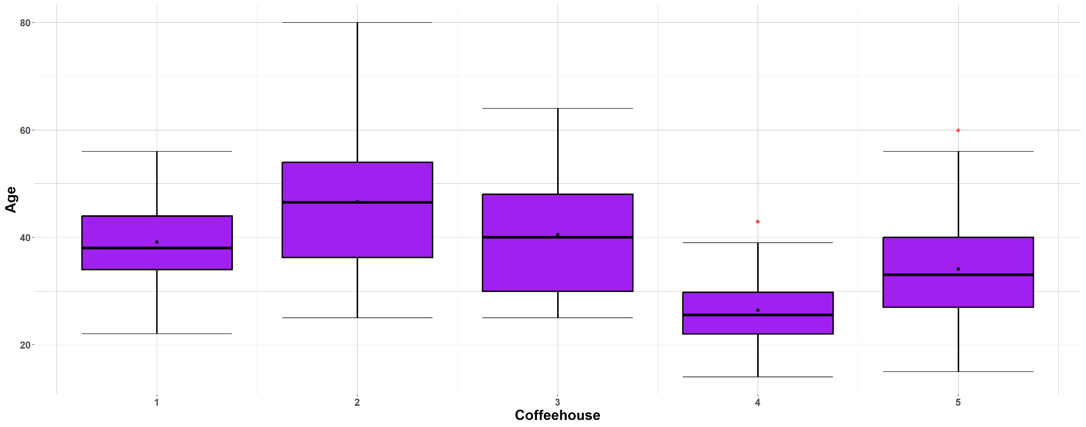
Fig. 12.2 Side-by-side boxplots of the five samples in the coffeehouse example

We assess the strength of visual evidence by how much the boxplots overlap in their spans. If all the boxplots span similar regions,there is little visual evidence of distinct means. If at least one group partially overlaps with the rest, there is a higher chance of eventually rejecting the null hypothesis in ANOVA.

Note that no formal conclusion should be drawn from visual evidence alone. Boxplots serve only as a tool to gain insight into the dataset.

Identifying Violation of Assumptions

This stage involves examining all available visual resources, including the boxplots, the histograms, and the normal probability plot.

(a) Boxplots

To confirm the equal variance assumption visually, ensure that the range and IQR of the samples are similar on the sid-by-side boxplots. The assumption must also be checked numerically. As a rule of thumb, we say that the sign of violation is not strong if:

\[\frac{\max{s_i}}{\min{s_i}} \leq 2.\]

Boxplots are also used to check if any potential outliers exist.

(b) Histograms and Normal Probability Plot

To check whether the samples show any signs of non-normality, use group-wise histograms.

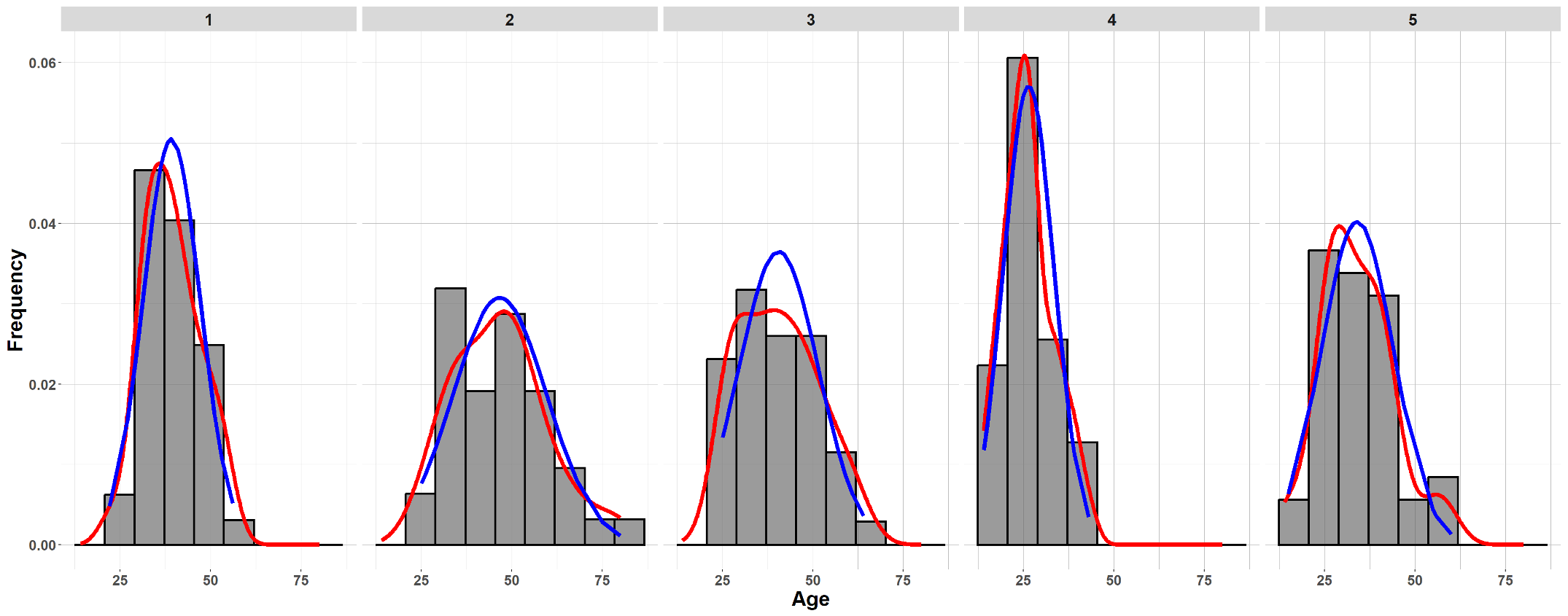
Fig. 12.3 Group-wise histograms for the coffeehouse example

A combined normal probability plot of \(x_{ij}-\bar{x}_{i\cdot}\) (data points re-centered to have zero-mean; also called the residuals) can be used together.

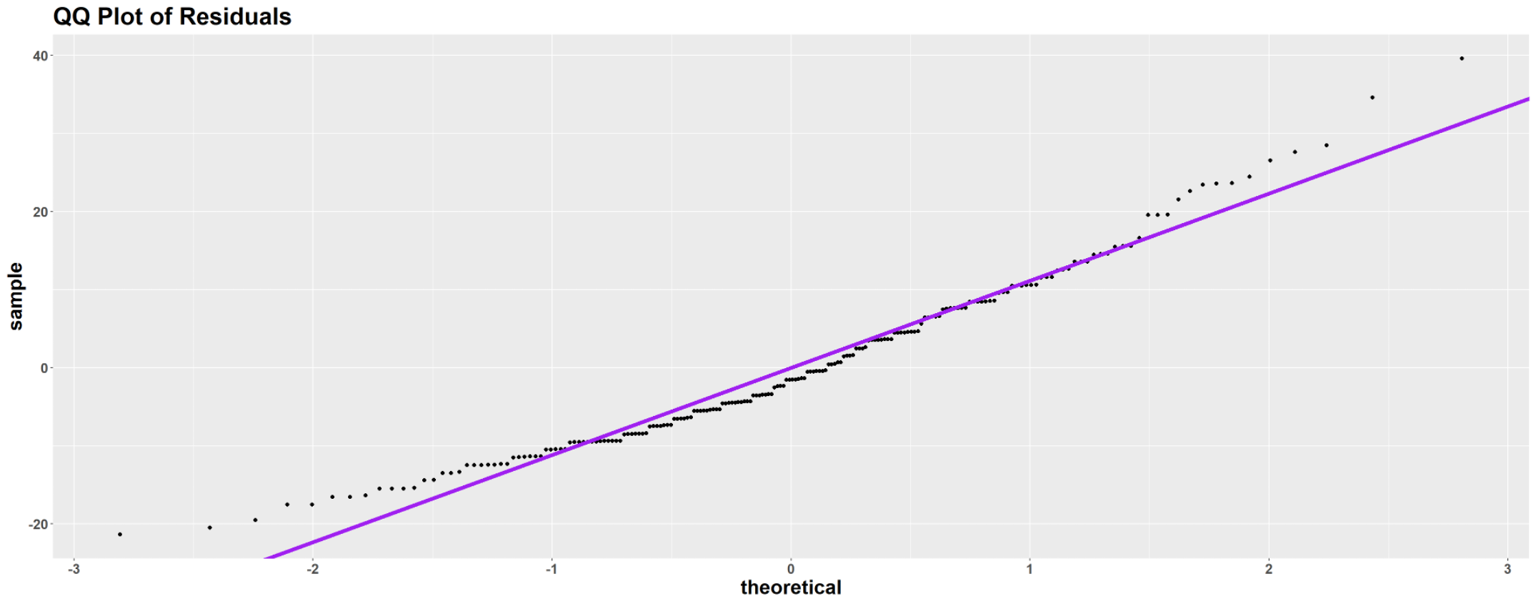
normal probability plot for the coffeehouse example — Fig. 12.4 Normal probability plot for the coffeehouse example

Example 💡: Coffeehouse Demographics Study ☕️

Use Fig. 12.2, Fig. 12.3, Fig. 12.4, and the numerical summary below to perform a preliminary assessment of the coffeehouse dataset.

📊 Download the coffeehouse dataset (CSV)

Table 12.1 Sample Statistics
Sample (Levels of Factor Variable)	Sample Size	Mean	Variance
Population 1	\(n_1 = 39\)	\(\bar{x}_{1.} = 39.13\)	\(s_1^2 = 62.43\)
Population 2	\(n_2 = 38\)	\(\bar{x}_{2.} = 46.66\)	\(s_2^2 = 168.34\)
Population 3	\(n_3 = 42\)	\(\bar{x}_{3.} = 40.50\)	\(s_3^2 = 119.62\)
Population 4	\(n_4 = 38\)	\(\bar{x}_{4.} = 26.42\)	\(s_4^2 = 48.90\)
Population 5	\(n_5 = 43\)	\(\bar{x}_{5.} = 34.07\)	\(s_5^2 = 98.50\)
Combined	\(n = 200\)	\(\bar{x}_{..} = 37.35\)	\(s^2 = 142.14\)

1. Do the graphs show signs of distinct means?

From the boxplots, we observe that the customer age sample from Coffeehouse 4 spans a notably lower region than others. Its difference with Coffeehouse 2 is most evident—the mean age at Coffeehouse 2 appears higher than even the maximum observed at Coffeehouse 4. Other coffeehouses show larger overlaps.

2. Any violation of assumptions?

Equal variance

From the boxplots, the variability of Sample 2 and Sample 4 appear to be different. We need to make sure that the largest ratio between two sample standard deviations is less than or equal to 2:

\[\frac{\max{s_i}}{\min{s_i}} = \frac{\sqrt{168.34}}{\sqrt{48.90}} = 1.855 < 2 \checkmark\]

So we consider the sample variances to be similar enough for the equal population variance assumption.

Normality

The histogram of Coffeehouse 4 and the overall QQ plot show a sign of skewness. Since the dataset is sufficiently large, this moderate departure from normality is okay.

3. Summary

Since the assumptions are reasonably met and the boxplots show signs of difference in means, we predict that ANOVA will yield a statistically significant result. We will perform the formal test in the upcoming sections and find out whether our prediction is correct.

Key Takeaways 📝

ANOVA is a statistical analysis that simultaneously compares two or more population means.
Double subscript notation \(X_{ij}\) systematically handles multiple groups, with dot notation indicating which indices are averaged over.
Four key assumptions must be satisfied for validity of ANOVA: independent simple random samples, independence between groups, normality, and equal variances.
Perform preliminary graphical and numerical assessments to check the assumptions and spot signs of statistical significance.

12.1.4. Exercises

Notation and Rounding Policy

Notation: In ANOVA, we use \(x_{i,j}\) where \(i\) indexes the group (1 to k) and \(j\) indexes the observation within that group. Always use a comma between subscripts to avoid ambiguity.

Rounding: Carry at least 3–4 decimal places in intermediate calculations; round final answers to 2 decimal places (or 3 significant figures for very small values like p-values).

Exercise 1: Identifying ANOVA Scenarios

For each scenario, determine whether one-way ANOVA is the appropriate analysis method. If not, suggest an alternative.

A software company compares bug detection rates of 4 different code review tools, testing each tool on 15 independent projects.
A researcher measures blood pressure before and after a meditation intervention for 30 participants.
An engineer compares the tensile strength of steel samples from 5 different suppliers, with 20 samples from each supplier.
A data scientist wants to determine if there’s a relationship between hours of sleep and exam scores.
A quality control team compares the precision of 3 measurement instruments by having each instrument measure the same 25 reference objects.
A marketing team tests whether click-through rates differ among 6 different ad designs, randomly showing each design to 500 users.

Exercise 2: Notation Practice

A materials engineer tests the hardness of ceramic samples produced using three different sintering temperatures. The following data are collected:

Temperature	Sample Size	Mean Hardness	Std Dev
1200°C (Group 1)	8	72.5	4.2
1350°C (Group 2)	10	78.3	3.8
1500°C (Group 3)	7	85.1	5.1

Notation convention: In ANOVA, we use double subscripts \(x_{i,j}\) where \(i\) indexes the group (1 to k) and \(j\) indexes the observation within that group (1 to \(n_i\)).

Using proper ANOVA notation, identify: \(k\), \(n_1, n_2, n_3\), \(n\), \(\bar{x}_{1.}, \bar{x}_{2.}, \bar{x}_{3.}\), \(s_1, s_2, s_3\).
Compute the overall (grand) mean \(\bar{x}_{..}\) using the formula:

\[\bar{x}_{..} = \frac{1}{n}\sum_{i=1}^{k} n_i \bar{x}_{i.}\]
What does the notation \(x_{2,5}\) represent in this context?
Write an expression for “the sum of all observations in Group 1” in two equivalent forms.

Exercise 3: Hypothesis Formulation

For each research scenario, write the null and alternative hypotheses using proper notation. Define the parameters clearly.

A network engineer tests whether mean packet latency differs among 4 different router configurations.
A pharmaceutical company compares the mean efficacy scores of 5 different drug dosages.
An agricultural researcher investigates whether mean crop yield differs among 3 fertilizer types.

Exercise 4: Checking the Equal Variance Assumption

The equal variance assumption is critical for valid ANOVA results. Use the rule of thumb: the assumption is reasonable if the ratio of the largest to smallest sample standard deviation is at most 2.

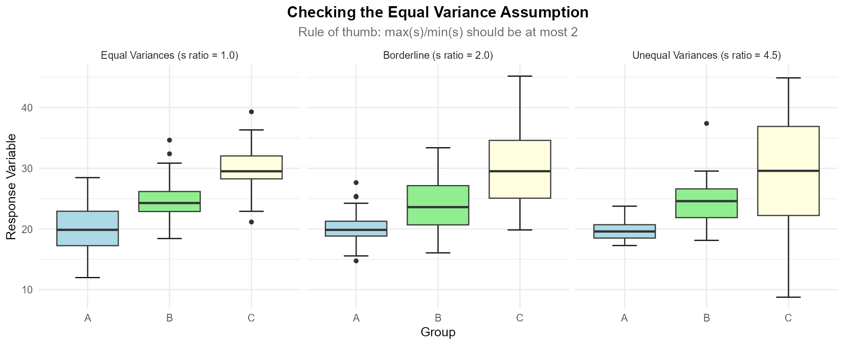
Equal vs unequal variance scenarios — Fig. 12.5 **Figure**: Side-by-side boxplots illustrating equal variances (left), borderline case (center), and unequal variances (right).

For each scenario, determine whether the equal variance assumption is satisfied.

Four treatment groups with sample standard deviations: \(s_1 = 12.4\), \(s_2 = 15.8\), \(s_3 = 11.2\), \(s_4 = 18.6\)
Three groups with sample variances: \(s_1^2 = 25\), \(s_2^2 = 81\), \(s_3^2 = 36\)
Five groups with the following summary:

Group

n

Mean

Variance

1

15

45.2

28.5

2

18

52.1

31.2

3

12

48.7

42.8

4

20

39.8

25.1

5

16

55.3

38.4

Exercise 5: Complete Assumption Checking with Plots

Before performing ANOVA inference, we must verify three key assumptions:

Independence (usually justified by study design)
Normality within each group (histograms, QQ-plots)
Equal variances across groups (boxplots, SD ratio)

A quality engineer collects tensile strength measurements (in MPa) from steel samples produced by three different manufacturing processes. The data is stored in a data frame called steel with variables Strength and Process (levels: A, B, C).

Write R code to create side-by-side boxplots with mean points to visually compare the three processes.
Write R code to create an effects plot showing the group means connected by lines.
Write R code to compute the sample size, mean, and standard deviation for each process using tapply().
Write R code to create faceted histograms by process with kernel density curves (red) and normal density overlays (blue).
Write R code to create faceted QQ-plots by process to assess normality within each group.
Check the equal variance assumption using the SD ratio rule of thumb.
Based on typical output from these plots, describe what you would look for to verify each assumption.

Example Output (for reference):

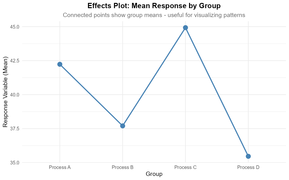
Example effects plot — Fig. 12.6 Effects plot showing group means connected by lines

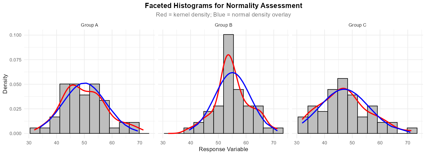
Example faceted histograms — Fig. 12.7 Faceted histograms with kernel density (red) and normal overlay (blue)

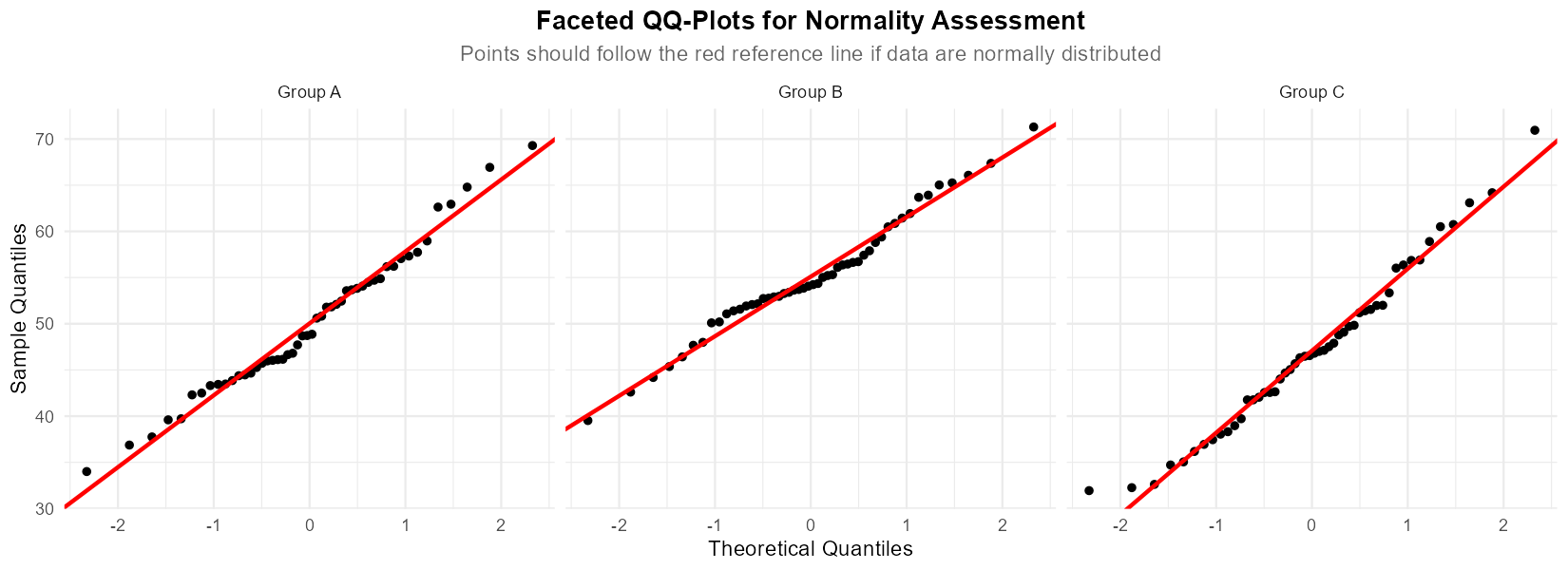
Example faceted QQ-plots — Fig. 12.8 Faceted QQ-plots for assessing normality within each group

Solution

Part (a): Side-by-side boxplots with mean points

library(ggplot2)

# Side-by-side boxplots
ggplot(steel, aes(x = Process, y = Strength)) +
  stat_boxplot(geom = "errorbar", width = 0.3) +
  geom_boxplot(fill = "lightblue") +
  stat_summary(fun = mean, geom = "point",
               color = "black", size = 3) +
  ggtitle("Tensile Strength by Manufacturing Process") +
  xlab("Process") +
  ylab("Tensile Strength (MPa)") +
  theme_minimal()

Part (b): Effects plot

# Effects plot - shows group means connected by lines
ggplot(steel, aes(x = Process, y = Strength)) +
  stat_summary(fun = mean, geom = "point", size = 3) +
  stat_summary(fun = mean, geom = "line", aes(group = 1)) +
  ggtitle("Effects Plot of Tensile Strength by Process") +
  xlab("Process") +
  ylab("Mean Tensile Strength (MPa)") +
  theme_minimal()

Part (c): Summary statistics using tapply()

# Sample sizes
n <- tapply(steel$Strength, steel$Process, length)

# Sample means
xbar <- tapply(steel$Strength, steel$Process, mean)

# Sample standard deviations
s <- tapply(steel$Strength, steel$Process, sd)

# Create summary table
summary_table <- data.frame(
  Process = names(n),
  n = as.numeric(n),
  Mean = round(xbar, 2),
  SD = round(s, 2)
)
print(summary_table)

Part (d): Faceted histograms with density overlays

# Calculate group statistics for normal density overlay
xbar <- tapply(steel$Strength, steel$Process, mean)
s <- tapply(steel$Strength, steel$Process, sd)

# Add normal density column to data frame
steel$normal.density <- mapply(function(value, group) {
  dnorm(value, mean = xbar[group], sd = s[group])
}, steel$Strength, steel$Process)

# Determine number of bins
n_bins <- max(round(sqrt(nrow(steel))) + 2, 5)

# Faceted histograms
ggplot(steel, aes(x = Strength)) +
  geom_histogram(aes(y = after_stat(density)),
                 bins = n_bins, fill = "grey", col = "black") +
  geom_density(col = "red", linewidth = 1) +
  geom_line(aes(y = normal.density), col = "blue", linewidth = 1) +
  facet_wrap(~ Process) +
  ggtitle("Histograms of Tensile Strength by Process") +
  xlab("Tensile Strength (MPa)") +
  ylab("Density") +
  theme_minimal()

Part (e): Faceted QQ-plots

# Add intercept and slope for QQ line (group-specific)
steel$intercept <- xbar[steel$Process]
steel$slope <- s[steel$Process]

# Faceted QQ-plots
ggplot(steel, aes(sample = Strength)) +
  stat_qq() +
  geom_abline(aes(intercept = intercept, slope = slope),
              color = "red", linewidth = 1) +
  facet_wrap(~ Process) +
  ggtitle("QQ Plots of Tensile Strength by Process") +
  xlab("Theoretical Quantiles") +
  ylab("Sample Quantiles") +
  theme_minimal()

Part (f): Equal variance check

# SD ratio rule of thumb
sd_ratio <- max(s) / min(s)
cat("SD ratio:", round(sd_ratio, 4), "\n")
cat("Equal variance assumption satisfied?",
    ifelse(sd_ratio <= 2, "Yes", "No"), "\n")

Part (g): What to look for in each plot

Side-by-side boxplots:

Equal variances: Boxes should have similar heights (IQRs) and whisker lengths
Separation of means: Look for overlap/separation between groups to predict ANOVA outcome
Outliers: Identify potential outliers (points beyond whiskers)

Effects plot:

Shows the pattern of group means clearly
Useful for predicting whether ANOVA will be significant
Large differences in height suggest group means differ

Faceted histograms:

Normality: Each histogram should be approximately bell-shaped
Kernel density (red) should roughly follow the normal density (blue)
Look for severe skewness or multimodality within groups

Faceted QQ-plots:

Normality: Points should fall approximately along the diagonal reference line
Deviations at tails: Suggest heavy or light tails
S-shaped pattern: Suggests skewness
Systematic curvature: Suggests non-normality

SD ratio:

If max(s)/min(s) ≤ 2, the equal variance assumption is reasonable
If ratio > 2, consider alternative methods (Welch’s ANOVA, beyond STAT 350)

Exercise 6: Interpreting Side-by-Side Boxplots

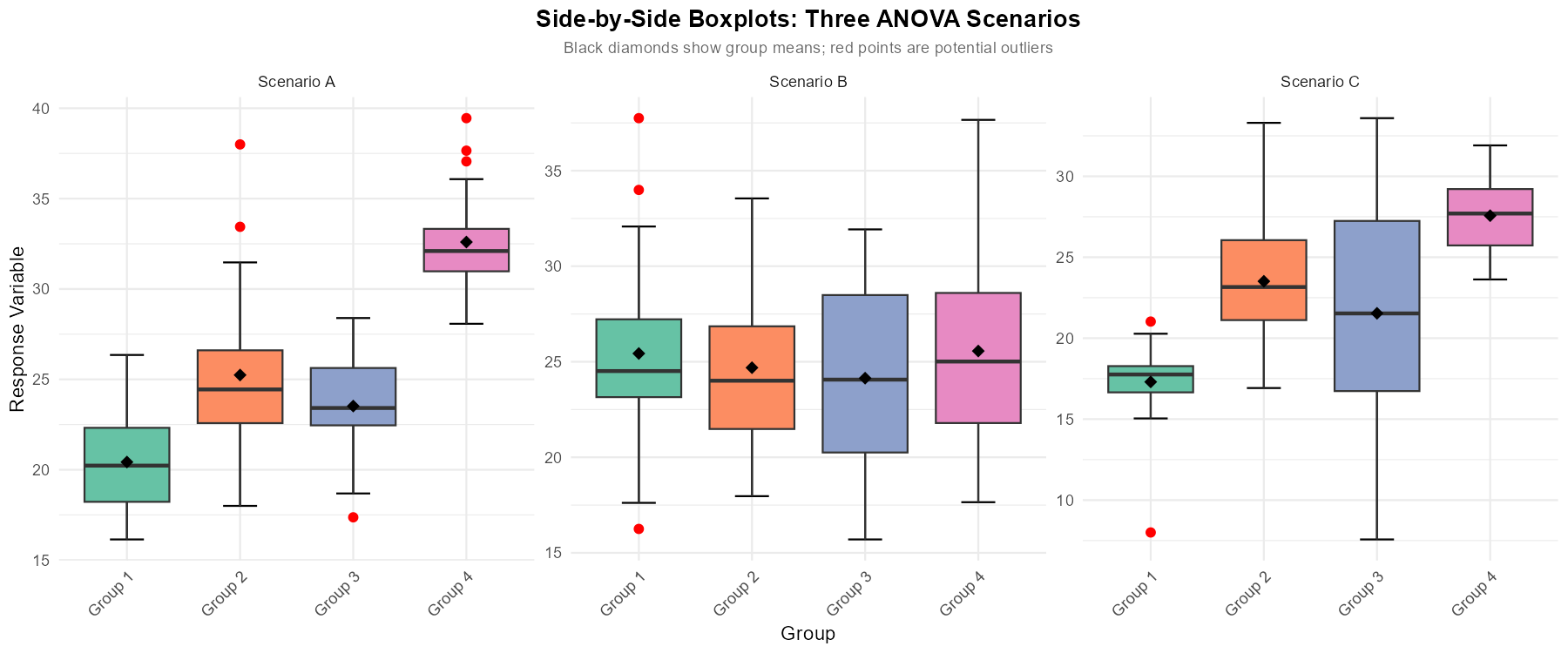
Side-by-side boxplots for three scenarios — Fig. 12.9 **Figure 1**: Side-by-side boxplots from three different studies comparing k = 4 groups.

For each scenario (A, B, C) shown in Figure 1:

Would you expect to reject \(H_0\) in the ANOVA F-test? Explain your reasoning based on the overlap of boxplots.
Are there any concerns about the equal variance assumption?
Are there any potential outliers that might affect the analysis?

Exercise 7: Why “Analysis of Variance”?

A common source of confusion is why a test for comparing means is called Analysis of Variance.

Explain in your own words why comparing variabilities (between-group vs. within-group) helps us determine whether population means differ.
Consider two scenarios with the same group sample means: \(\bar{x}_1 = 10\), \(\bar{x}_2 = 15\), \(\bar{x}_3 = 20\). In Scenario I, each group has \(s = 2\). In Scenario II, each group has \(s = 8\). Which scenario provides stronger evidence that the population means differ? Explain.
If \(H_0: \mu_1 = \mu_2 = ... = \mu_k\) is true, what would you expect the ratio MSA/MSE to be approximately equal to? Why?

Exercise 8: The Multiple Testing Problem

A researcher wants to compare mean response times across k = 5 different algorithm implementations.

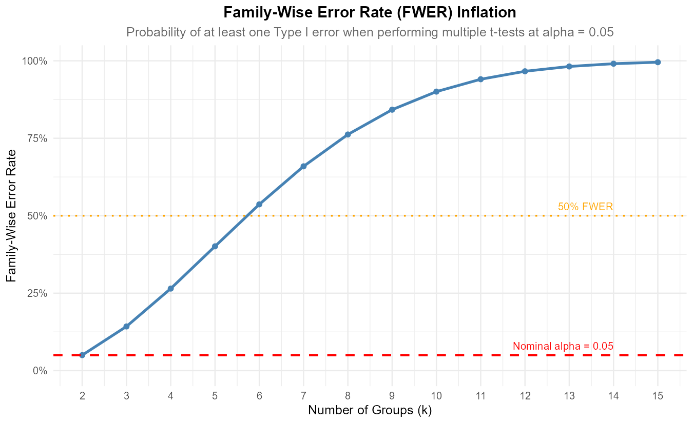
Family-wise error rate inflation — Fig. 12.10 **Figure**: Family-wise error rate (FWER) increases rapidly with the number of groups when using multiple t-tests at α = 0.05.

How many pairwise comparisons would be needed to compare all pairs of algorithms?
If the researcher performs each pairwise comparison as a separate two-sample t-test at α = 0.05, what is the probability of making at least one Type I error (assuming all null hypotheses are true and tests are independent)?
Why does ANOVA provide a better approach than multiple t-tests?
For k = 10 groups, how many pairwise comparisons are needed? What would the family-wise error rate be if using individual α = 0.05 tests?

Exercise 9: True/False Conceptual Questions

Determine whether each statement is True or False. Provide a brief justification.

In ANOVA, if we reject \(H_0\), we can conclude that all population means are different from each other.
The ANOVA F-test requires that all group sample sizes be equal.
If the boxplots for all groups show similar medians but very different spreads, the equal variance assumption may be violated.
The alternative hypothesis in one-way ANOVA can be directional (e.g., \(\mu_1 < \mu_2 < \mu_3\)).
If sample sizes are large (n > 40 per group), ANOVA is robust to moderate departures from normality.
ANOVA with k = 2 groups is equivalent to a two-sample t-test under certain conditions.

Exercise 10: Designing an ANOVA Study

A biomedical engineering team wants to compare the effectiveness of 4 different stent designs in maintaining arterial blood flow. They plan to conduct an experiment using a laboratory flow simulation system.

Identify the factor variable and its levels.
Identify an appropriate quantitative response variable.
Write the null and alternative hypotheses.
What sample size considerations should the team address?
How could the team ensure the independence assumption is satisfied?
What potential issues might arise with the equal variance assumption, and how could they check it?

12.1.5. Additional Practice Problems

True/False Questions (1 point each)

The ANOVA F-test can determine which specific group means are different from each other.

Ⓣ or Ⓕ
If all sample means are identical (\(\bar{x}_1 = \bar{x}_2 = ... = \bar{x}_k\)), the F-test statistic will equal exactly 0.

Ⓣ or Ⓕ
The notation \(\bar{x}_{3.}\) represents the mean of the third observation across all groups.

Ⓣ or Ⓕ
ANOVA assumes that each group is sampled independently from its respective population.

Ⓣ or Ⓕ
If an ANOVA study has k = 6 groups with 10 observations each, the total sample size is n = 60.

Ⓣ or Ⓕ
The equal variance assumption can be checked by computing the ratio of the largest to smallest sample standard deviations.

Ⓣ or Ⓕ

Multiple Choice Questions (2 points each)

In ANOVA notation, \(x_{2,7}\) represents:

Ⓐ The 2nd observation in the 7th group

Ⓑ The 7th observation in the 2nd group

Ⓒ The product of 2 and 7

Ⓓ The sum of observations in groups 2 and 7
For a study comparing k = 4 groups, the alternative hypothesis is:

Ⓐ \(H_a: \mu_1 \neq \mu_2 \neq \mu_3 \neq \mu_4\)

Ⓑ \(H_a: \mu_1 = \mu_2 = \mu_3 = \mu_4\)

Ⓒ \(H_a:\) At least one \(\mu_i\) is different from the others

Ⓓ \(H_a: \mu_1 > \mu_2 > \mu_3 > \mu_4\)
Which is NOT an assumption of one-way ANOVA?

Ⓐ Independent random samples from each population

Ⓑ Normal distributions (or large samples)

Ⓒ Equal population variances

Ⓓ Equal sample sizes from each population
The rule of thumb for checking equal variances requires:

Ⓐ \(\max(s_i^2)/\min(s_i^2) \leq 2\)

Ⓑ \(\max(s_i)/\min(s_i) \leq 2\)

Ⓒ \(\max(\bar{x}_i)/\min(\bar{x}_i) \leq 2\)

Ⓓ All sample variances within 2 units of each other
The overall sample mean \(\bar{x}_{..}\) is calculated as:

Ⓐ The simple average of group means

Ⓑ A weighted average of group means, weighted by sample sizes

Ⓒ The median of all observations

Ⓓ The sum of all group means

Group	n	Mean	Variance
1	15	45.2	28.5
2	18	52.1	31.2
3	12	48.7	42.8
4	20	39.8	25.1
5	16	55.3	38.4