Slides 📊

Download Chapter 9 slides (PPTX)

9.2. Confidence Intervals for the Population Mean, When σ is Known

Confidence intervals are one of the most fundamental tools for expressing uncertainty around a point estimate. In this section, we focus on constructing the confidence interval for a population mean \(\mu\) when the population standard deviation \(\sigma\) is known. While this scenario is somewhat rare in practice (as \(\sigma\) is typically unknown), it provides a clear foundation for understanding the core logic of interval estimation.

Road Map 🧭

• Understand the complementary roles of a point estimator and an interval estimator.

• Derive the confidence interval for a population mean \(\mu\), given that the population standard deviation \(\sigma\) is known. Apply the derived formula to problems.

• Understand the difference between a confidence interval as an estimator and and a realized estimate, and correctly interpret each.

9.2.1. Why Point Estimates Aren’t Enough

In practice, we usually have access to only one sample from the population. When we use a point estimator \(\hat{\theta}\) to estimate a parameter \(\theta\), we obtain only one realization out of many potential estiamtes that could have been observed. From this alone, we do not know how precise our current estimate is.

To address this limitation, we turn to an interval estimator, which relies on the sampling distribution of \(\hat{\theta}\) to measure and express uncertainty.

Interval Estimators

An interval estimator of a parameter \(\theta\) aims to provide a range of possible values for its true location. It is typically constructed by expanding left and right from a point estimator. For a point estimator \(\hat{\theta}\) whose sampling distirbution is symmetric, the expansion is also symmetric. That is, it takes the following general form:

\[(\hat{\theta} - ME, \hat{\theta} + ME),\]

where ME stands for the margin of error. The margin of error expresses the magnitude of expansion from the reference point, and therefore is always non-negative. Its value is determined by a combination of several components, such as

• The population distribution,

• The definition of the point estimator \(\hat{\theta}\), and

• The sample size \(n\).

9.2.2. Confidence Interval for \(\mu\), When \(\sigma\) is Known

We now construct a specific class of interval estimators for the population mean \(\mu\), based on its most widely used point estimator \(\bar{X}\). This class is called Confidence Intervals (CIs).

The Goal

For a pre-specified value \(C\) between 0 and 1, a confidence interval for \(\mu\) aims to capture \(\mu\) with probability \(C\). Mathematically, this is equivalent to finding the ME (margin of error) which satisfies:

\[P\left(\bar{X}-ME < \mu < \bar{X} + ME \right) = C.\]

Preliminaries

Before diving into the main derivation, let us first touch on its key ingredients.

• The probability \(C\) is called the confidence coefficient of a confidence interval.

• When expressed in the percentage scale, \(C \cdot 100\%\) is called the confidence level of a confidence interval.

• We denote the complement of \(C\) as \(\alpha\). That is,

  \[\alpha = 1 - C.\]

• Another important ingredient is the \(z\)-critical value. A \(z\)-critical value \(z_{\alpha/2}\) is the value on a standard normal pdf which marks an upper area of \(\alpha/2\).

  

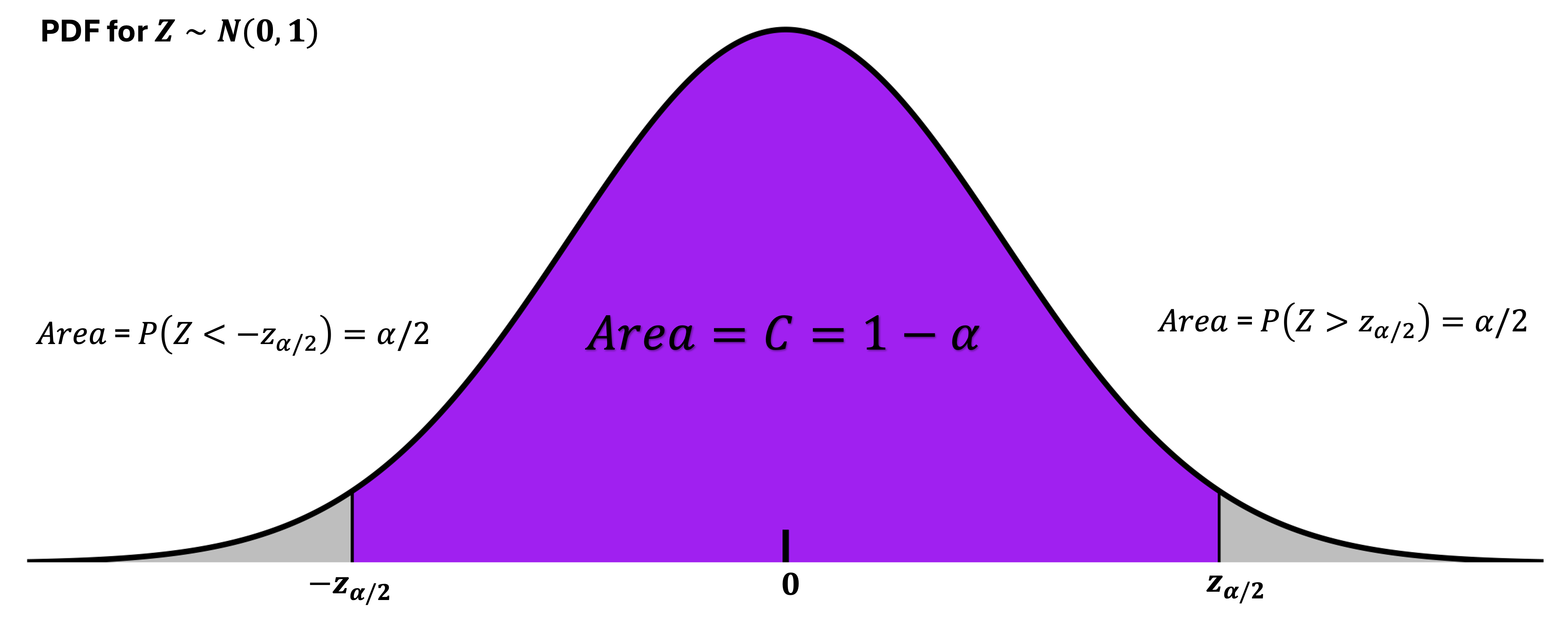
  By the symmetry of the standard normal distribution around 0, the region below \(-z_{\alpha/2}\) also has the area \(\alpha/2\). Note that this leaves the central region bewteen \(-z_{\alpha/2}\) and \(z_{\alpha/2}\) exactly the area of \(C\).

Deriving the Confidence Interval: The Pivotal Method

This derivation is valid under the following assumptions:

1. \(X_1, X_2, \ldots, X_n\) form an iid sample from the population, \(X\). The expected value and variance of \(X\) is denoted \(\mu\) and \(\sigma^2\), respectively.

2. Either the population is normally distributed, or we have sufficiently large \(n\) for the CLT to hold.

3. The population variance \(\sigma^2\) is known.

From the first and second assumptions, we have:

\[\bar{X} \sim N\left(\mu, \frac{\sigma^2}{n}\right),\]

which is equivalent to stating that its standardization has a standard normal distribution:

\[\frac{\bar{X} - \mu}{\sigma/\sqrt{n}} \sim N(0, 1).\]

The standardization of \(\bar{X}\) is also called the pivotal quantity. We are now ready to take the final steps.

Step 1: Find the Interval Under the Standard Normal Distribution

From the preliminaries, we already know that

\[P\left(-z_{\alpha/2} < Z < z_{\alpha/2}\right) = C.\]

Step 2: Replace \(Z\) with the Pivotal Quantity

\[P\left(-z_{\alpha/2} < \frac{\bar{X} - \mu}{\sigma/\sqrt{n}} < z_{\alpha/2}\right) = C.\]

This is possible because the pivotal quantity has the same distribution as \(Z\).

Step 3: Rearrange the Inequalities

1. Multiply all terms by \(\frac{\sigma}{\sqrt{n}}\):

   \[P\left(-z_{\alpha/2} \frac{\sigma}{\sqrt{n}} < \bar{X} - \mu < z_{\alpha/2} \frac{\sigma}{\sqrt{n}}\right) = C\]

2. Multiply by -1 and reverse the inequalities:

   \[P\left(z_{\alpha/2} \frac{\sigma}{\sqrt{n}} > \mu - \bar{X} > -z_{\alpha/2} \frac{\sigma}{\sqrt{n}}\right) = C\]

3. Rearrange to isolate \(\mu\):

   \[P\left(\bar{X} - z_{\alpha/2} \frac{\sigma}{\sqrt{n}} < \mu < \bar{X} + z_{\alpha/2} \frac{\sigma}{\sqrt{n}}\right) = C\]

At this point, the probability statement looks exactly like our goal, with a computable representation of the ME.

Summary

From the result above, we discover that the margin of error for the \(C\cdot 100 \%\) confidence interval of \(\mu\) is

\[ME = z_{\alpha/2}\frac{\sigma}{\sqrt{n}}.\]

Plugging this into the general form, we finally obtain the complete expression for the confidence interval:

\[\left(\bar{X} - z_{\alpha/2} \frac{\sigma}{\sqrt{n}}, \bar{X} + z_{\alpha/2} \frac{\sigma}{\sqrt{n}}\right).\]

Alternatively, the CI is also written as:

\[\bar{X} \pm z_{\alpha/2} \frac{\sigma}{\sqrt{n}}.\]

Confidence Interval Is Also a Random Variable‼️

Note that a confidence interval will also vary from sample to sample, since its center, \(\bar{X}\), does. This means that we can view a CI as a (bivariate) random variable.

In practice, we have one realization of a CI based on a single sample:

\[\left(\bar{x} - z_{\alpha/2} \frac{\sigma}{\sqrt{n}}, \bar{x} + z_{\alpha/2} \frac{\sigma}{\sqrt{n}}\right).\]

Note that the center is now represented with the lower case \(\bar{x}\). Unlike a point estimate, however, a realized CI still gives us a measure of precision through its width. A narrow interval suggests high precision, while a wide interval reflects greater uncertainty.

New Terminology: Standard Error

To distinguish from the population standard deviation \(\sigma\), we often call the true standard deviation of an estimator the standard error.

In our current setting, the standard error is \(\sigma_{\bar{X}} = \sigma/\sqrt{n}\). However, the mathematical definition of a standard error changes by the inference problem and its appropriate point estimator. We will encounter a few different standard errors in the upcoming chapters.

Example 💡: American Adult Male Weights

Historical data from 1960 indicated that the weight of American adult males was normally distributed with a mean of \(\mu = 166.3\) lbs and a standard deviation of \(\sigma = 49.26\) lbs.

In 2000, researchers collected a new sample of \(n = 3,791\) adult males and found a sample mean of \(\bar{x} = 191\) lbs. Assuming the standard deviation hasn’t changed, compute a 99% confidence interval for the mean weight of American adult males in 2000.

The building blocks

• Sample mean: \(\bar{x} = 191\) lbs

• Population standard deviation: \(\sigma = 49.26\) lbs

• Sample size: \(n = 3,791\)

• Confidence level: \(99\% \, (C = 0.99, \alpha = 0.01)\)

Find the critical value

The critical value: \(z_{\alpha/2} = z_{0.005}\) is equal to the 99.5th percentile of a standard normal distribution. You can use the R command:

qnorm(0.005, lower.tail=FALSE)

We find that \(z_{0.005} = 2.5758\).

Find the margin of error

\[\text{ME} = z_{0.005} \frac{\sigma}{\sqrt{n}} = 2.5758 \frac{49.26}{\sqrt{3791}} \approx 2.06 \text{ lbs}\]

Construct the confidence interval

\[\bar{x} \pm \text{ME} = 191 \pm 2.06 = [188.94 \text{ lbs}, 193.06 \text{ lbs}]\]

9.2.3. Interpreting Confidence Intervals Correctly

Suppose a 95% confidence interval of \((121.4, 126.2)\) is computed for the true mean crop yield of corn in a certain state, in bushels per acre. Then, it is incorrect to interpret the numbers as the following:

❌ “With 0.95 probability, the true mean yield of corn is between 121.4 and 126.2 bushels per acre.” ❌

The statement is incorrect for two main reasons, which we now analyze one by one.

Common Pitfall 1: Probabilities of a Confidence Interval

The confidence interval was constructed so that its probability of including the true mean is 0.95. However, this property is true for the CI as an estimator, which is a random variable, NOT for a set of realized values. Once the upper and lower values are determined as \((121.4, 126.2)\), they do not have any probabilistic relationship with another fixed quantity, \(\mu\). Therefore, the expression “With 0.95 probability…” is inaccurate.

Common Pitfall 2: Interval Is Random, \(\mu\) Is Not

Since a realized confidence interval is observed while the population mean \(\mu\) is not, it is easy to mistakenly imply that \(\mu\) varies from sample to sample, rather than the interval itself. The incorrect statement above implies that the true mean yield of corn either succeeds or fails to be between the two fixed numbers, which is not accurate.

We should always remember that \(\mu\) is an unknown yet unchanging property of the population distribution, whereas the confidence interval changes from sample to sample. Our interpretations should reflect this distinction as accurately as possible.

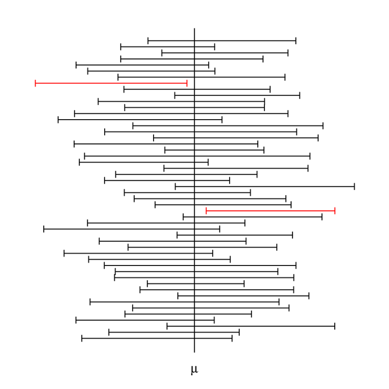
Fig. 9.3 \(\mu\) stays fixed while the confidence interval changes over different samples.

How To Say It Better

To include the confidence level as part of the interpretation, we use the term “confidence.” We say

✅ With 95% confidence, the interval \((121.4, 126.2)\) captures the true mean yield of corn. ✅

Confidence here is not used in its everyday sense, but as a technical term. It means that \((121.4, 126.2)\) is one realization of a random variable which, across many samples, successfully captures the true mean with probability 0.95.

It is also possible to interpret \(C\) as a probability, provided that the discussion is focused on the confidence interval as a random variable. It is correct to say

✅ Over many computations of the CI using different samples, the probability that it captures \(\mu\) is approximately 0.95. ✅

Here, 0.95 indicates the proportion of “successful” CIs out of the complete collection of a very large number of computed CIs.

Confidence Intervals Simulation 🎮

Explore how confidence intervals behave by generating images like Fig. 9.3 under different population distributions, sample sizes, and confidence level.

🔗 Launch Interactive Demo | 📄 View R Code

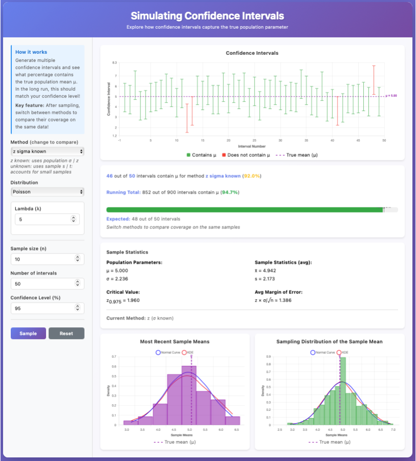
Fig. 9.4 CI simulator preview

Templates for Valid Interpretations

You are encouraged to use the templates below for interpretations of confidence intervals. Simply replace the parentheses with specific values/contexts from your experiment.

Templates for Interpreting a CI
Case	Template
When interpreting a concrete outcome of an experiment (an interval estimate)	With (\(C \cdot 100\))% confidence, the interval (lower value, upper value) captures the true/population mean of (context).
When interpreting a CI as an interval estimator	Over many repeated trials of (experiment context), the proportion of realized confidence intervals which capture the true mean of (context) will be about (\(C\)).

Example 💡: American Adult Male Weights, Continued

In the previous example, we computed a 99% confidence interval for the true mean weight of American adult males as \([188.94, 193.06]\). Give a valid interpretation of this outcome.

Interpretation: We are 99% confident that the interval between 188.94 and 193.06 pounds includes the true mean weight of American adult males in 2000.

9.2.4. Bringing It All Together

Key Takeaways 📝

• An interval estimator provides a range of plausible values for a population parameter.

• For a population mean with known standard deviation, its confidence interval is defined as \(\bar{X} \pm z_{\alpha/2} \frac{\sigma}{\sqrt{n}}\).

• A confidence interval from a single experiment should be interpreted with care. Once a set of realized values, its interpretation should not directly involve any probabilities. Use the term confidence to imply its generation procedure.

Learning Objectives 🎯

These exercises will help you:

• Find z-critical values for various confidence levels

• Construct confidence intervals for the population mean when σ is known

• Calculate and interpret the margin of error

• Correctly interpret confidence intervals (avoiding common misconceptions)

• Understand the probabilistic meaning of confidence level

Key Formulas 📐

Confidence Interval for μ (σ known):

\[\bar{x} \pm z_{\alpha/2} \frac{\sigma}{\sqrt{n}}\]

Margin of Error:

\[ME = z_{\alpha/2} \frac{\sigma}{\sqrt{n}}\]

R Functions:

# z-critical value for confidence level C
alpha <- 1 - C
qnorm(alpha/2, lower.tail = FALSE)

# Common values
qnorm(0.05, lower.tail = FALSE)   # 90% CI: z = 1.645
qnorm(0.025, lower.tail = FALSE)  # 95% CI: z = 1.960
qnorm(0.005, lower.tail = FALSE)  # 99% CI: z = 2.576

9.2.5. Exercises

Exercise 1: Finding z-Critical Values

Find the z-critical value \(z_{\alpha/2}\) for each confidence level. Use R or a standard normal table.

1. 90% confidence level

2. 95% confidence level

3. 99% confidence level

4. 98% confidence level

5. 80% confidence level

Solution

Finding z-critical values using \(z_{\alpha/2}\):

Part (a): 90% CI (\(\alpha = 0.10\), \(\alpha/2 = 0.05\))

qnorm(0.05, lower.tail = FALSE)  # 1.6449

\(z_{0.05} = 1.645\)

Part (b): 95% CI (\(\alpha = 0.05\), \(\alpha/2 = 0.025\))

qnorm(0.025, lower.tail = FALSE)  # 1.9600

\(z_{0.025} = 1.960\)

Part (c): 99% CI (\(\alpha = 0.01\), \(\alpha/2 = 0.005\))

qnorm(0.005, lower.tail = FALSE)  # 2.5758

\(z_{0.005} = 2.576\)

Part (d): 98% CI (\(\alpha = 0.02\), \(\alpha/2 = 0.01\))

qnorm(0.01, lower.tail = FALSE)  # 2.3263

\(z_{0.01} = 2.326\)

Part (e): 80% CI (\(\alpha = 0.20\), \(\alpha/2 = 0.10\))

qnorm(0.10, lower.tail = FALSE)  # 1.2816

\(z_{0.10} = 1.282\)

---

Exercise 2: Basic CI Construction

A quality engineer measures the diameter of precision ball bearings from a production line. Based on a random sample of \(n = 36\) ball bearings, the sample mean diameter is \(\bar{x} = 5.02\) mm. Historical data indicate the population standard deviation is \(\sigma = 0.08\) mm.

1. Calculate the standard error of the sample mean.

2. Find the z-critical value for a 95% confidence interval.

3. Calculate the margin of error.

4. Construct the 95% confidence interval for the true mean diameter.

5. Interpret the confidence interval in the context of the problem.

Solution

Given: \(n = 36\), \(\bar{x} = 5.02\) mm, \(\sigma = 0.08\) mm

Part (a): Standard error

\[SE = \frac{\sigma}{\sqrt{n}} = \frac{0.08}{\sqrt{36}} = \frac{0.08}{6} = 0.01333 \text{ mm}\]

Part (b): z-critical value

For 95% CI: \(z_{0.025} = 1.960\)

Part (c): Margin of error

\[ME = z_{0.025} \times SE = 1.960 \times 0.01333 = 0.02613 \text{ mm}\]

Part (d): 95% confidence interval

\[\bar{x} \pm ME = 5.02 \pm 0.026 = (4.994, 5.046) \text{ mm}\]

Part (e): Interpretation

We are 95% confident that the true mean diameter of ball bearings from this production line is between 4.994 mm and 5.046 mm.

R verification:

xbar <- 5.02; sigma <- 0.08; n <- 36
SE <- sigma / sqrt(n)
z_crit <- qnorm(0.025, lower.tail = FALSE)
ME <- z_crit * SE
c(xbar - ME, xbar + ME)  # [4.9939, 5.0461]

---

Exercise 3: Network Latency Analysis

A network engineer monitors response times for a web application. From a sample of \(n = 49\) requests, the sample mean response time is \(\bar{x} = 245\) ms. The population standard deviation is known to be \(\sigma = 35\) ms from long-term monitoring.

1. Construct a 90% confidence interval for the true mean response time.

2. Construct a 99% confidence interval for the true mean response time.

3. Which interval is wider? Explain why this makes sense.

4. If the service level agreement requires a mean response time below 260 ms, what do your intervals suggest?

Solution

Given: \(n = 49\), \(\bar{x} = 245\) ms, \(\sigma = 35\) ms

Standard error: \(SE = \frac{35}{\sqrt{49}} = \frac{35}{7} = 5\) ms

Part (a): 90% CI (\(z_{0.05} = 1.645\))

\[ME = 1.645 \times 5 = 8.225 \text{ ms}\]

\[CI: 245 \pm 8.23 = (236.78, 253.22) \text{ ms}\]

Part (b): 99% CI (\(z_{0.005} = 2.576\))

\[ME = 2.576 \times 5 = 12.88 \text{ ms}\]

\[CI: 245 \pm 12.88 = (232.12, 257.88) \text{ ms}\]

Part (c): Width comparison

The 99% CI is wider (width = 25.76 ms vs 16.45 ms). This makes sense because higher confidence requires casting a wider net to increase the probability of capturing the true parameter.

Part (d): SLA evaluation

Both intervals have upper bounds well below 260 ms (253.22 and 257.88 respectively). This provides evidence that the mean response time meets the SLA requirement of being below 260 ms.

R verification:

xbar <- 245; sigma <- 35; n <- 49
SE <- sigma / sqrt(n)  # 5

# 90% CI
z90 <- qnorm(0.05, lower.tail = FALSE)
c(xbar - z90*SE, xbar + z90*SE)  # [236.78, 253.22]

# 99% CI
z99 <- qnorm(0.005, lower.tail = FALSE)
c(xbar - z99*SE, xbar + z99*SE)  # [232.12, 257.88]

---

Exercise 4: Identifying Correct Interpretations

A researcher constructs a 95% confidence interval of (72.4, 78.6) for the mean score on a standardized test.

For each statement below, indicate whether it is a CORRECT or INCORRECT interpretation. Explain why.

1. “We are 95% confident that the true mean score is between 72.4 and 78.6.”

2. “There is a 95% probability that the true mean score lies between 72.4 and 78.6.”

3. “95% of all students scored between 72.4 and 78.6.”

4. “If we repeated this study many times, approximately 95% of the resulting confidence intervals would contain the true mean.”

5. “The sample mean is 75.5 with 95% certainty.”

6. “We are 95% confident that the interval (72.4, 78.6) captures the true population mean score.”

Solution

CI: (72.4, 78.6) at 95% confidence

Part (a): “We are 95% confident that the true mean score is between 72.4 and 78.6.”

CORRECT ✓ – This is the standard proper interpretation using “confidence.”

Part (b): “There is a 95% probability that the true mean score lies between 72.4 and 78.6.”

INCORRECT ✗ – Once the interval is calculated, μ either is or isn’t in it (μ is fixed). Probability applies to the procedure, not to a specific realized interval.

Part (c): “95% of all students scored between 72.4 and 78.6.”

INCORRECT ✗ – The CI estimates the population mean, not individual scores. Individual scores have much more variability than the sample mean.

Part (d): “If we repeated this study many times, approximately 95% of the resulting confidence intervals would contain the true mean.”

CORRECT ✓ – This correctly describes the frequentist interpretation of confidence level.

Part (e): “The sample mean is 75.5 with 95% certainty.”

INCORRECT ✗ – The sample mean is known exactly (\(\bar{x} = 75.5\)); there’s no uncertainty about the sample mean itself. The uncertainty is about the population mean μ.

Part (f): “We are 95% confident that the interval (72.4, 78.6) captures the true population mean score.”

CORRECT ✓ – Equivalent to (a), properly emphasizing that the interval (not μ) is what varies.

Note on frequentist vs. Bayesian interpretation: In the frequentist CI we use in this course, μ is treated as a fixed (but unknown) constant, and the interval is random. The 95% refers to the long-run success rate of the procedure. In Bayesian inference (not covered in this course), probability statements about μ itself are possible, but they come from a posterior distribution based on prior beliefs and data.

---

Exercise 5: Effect of Sample Size on CI

A pharmaceutical company is testing the dissolution rate of a new tablet formulation. The population standard deviation is known to be \(\sigma = 4.2\) mg/min from previous formulations.

A pilot study with \(n = 16\) tablets yields \(\bar{x} = 28.5\) mg/min.

1. Construct a 95% confidence interval using \(n = 16\).

2. Suppose the company increases the sample size to \(n = 64\). Using the same \(\bar{x} = 28.5\), construct a new 95% CI.

3. By what factor did the margin of error decrease when \(n\) increased from 16 to 64?

4. What sample size would be needed to achieve a margin of error of 1.0 mg/min at 95% confidence?

Solution

Given: \(\sigma = 4.2\) mg/min, \(\bar{x} = 28.5\) mg/min

Part (a): 95% CI with n = 16

\[SE = \frac{4.2}{\sqrt{16}} = \frac{4.2}{4} = 1.05 \text{ mg/min}\]

\[ME = 1.96 \times 1.05 = 2.058 \text{ mg/min}\]

\[CI: 28.5 \pm 2.06 = (26.44, 30.56) \text{ mg/min}\]

Part (b): 95% CI with n = 64

\[SE = \frac{4.2}{\sqrt{64}} = \frac{4.2}{8} = 0.525 \text{ mg/min}\]

\[ME = 1.96 \times 0.525 = 1.029 \text{ mg/min}\]

\[CI: 28.5 \pm 1.03 = (27.47, 29.53) \text{ mg/min}\]

Part (c): Factor of decrease

\[\frac{ME_{n=16}}{ME_{n=64}} = \frac{2.058}{1.029} = 2\]

The ME decreased by a factor of 2. This equals \(\sqrt{64/16} = \sqrt{4} = 2\).

Part (d): Required n for ME = 1.0 mg/min

\[1.0 = 1.96 \times \frac{4.2}{\sqrt{n}}\]

\[\sqrt{n} = \frac{1.96 \times 4.2}{1.0} = 8.232\]

\[n = 67.77 \Rightarrow n^* = 68\]

Need at least n = 68 tablets.

---

Exercise 6: CPU Temperature Monitoring

A data center engineer monitors CPU temperatures during peak load. From extensive historical data, the population standard deviation is \(\sigma = 8.5°C\). A random sample of \(n = 50\) measurements during a stress test yields \(\bar{x} = 72.3°C\).

1. Construct a 95% confidence interval for the mean CPU temperature during peak load.

2. The manufacturer specifies that the mean operating temperature should not exceed 75°C. Based on your interval, is there evidence that the mean temperature is within specification?

3. If the engineer wants to be more certain, construct a 99% confidence interval. Does the conclusion change?

Solution

Given: \(\sigma = 8.5°C\), \(n = 50\), \(\bar{x} = 72.3°C\)

\(SE = \frac{8.5}{\sqrt{50}} = 1.202°C\)

Part (a): 95% CI

\[ME = 1.96 \times 1.202 = 2.36°C\]

\[CI: 72.3 \pm 2.36 = (69.94, 74.66)°C\]

Part (b): Specification check (95% CI)

The entire 95% CI is below 75°C. This provides evidence that the mean temperature is within the manufacturer’s specification.

Part (c): 99% CI

\[ME = 2.576 \times 1.202 = 3.10°C\]

\[CI: 72.3 \pm 3.10 = (69.20, 75.40)°C\]

The 99% CI extends slightly above 75°C (upper bound = 75.40). At this higher confidence level, we cannot be certain the specification is met. The conclusion is less definitive.

R verification:

xbar <- 72.3; sigma <- 8.5; n <- 50
SE <- sigma / sqrt(n)  # 1.202

# 95% CI
z95 <- qnorm(0.025, lower.tail = FALSE)
c(xbar - z95*SE, xbar + z95*SE)  # [69.94, 74.66]

# 99% CI
z99 <- qnorm(0.005, lower.tail = FALSE)
c(xbar - z99*SE, xbar + z99*SE)  # [69.20, 75.40]

---

Exercise 7: Comparing Different Confidence Levels

Using the data from Exercise 6 (\(\bar{x} = 72.3\), \(\sigma = 8.5\), \(n = 50\)), construct confidence intervals at the following levels:

1. 80% confidence level

2. 90% confidence level

3. 95% confidence level

4. 99% confidence level

5. Create a table showing the confidence level, z-critical value, margin of error, and interval bounds. What pattern do you observe?

Solution

Given: \(\bar{x} = 72.3\), \(\sigma = 8.5\), \(n = 50\), \(SE = 1.202\)

Table 9.1 Confidence Intervals at Different Levels

Conf. Level	\(z_{\alpha/2}\)	ME	Lower Bound	Upper Bound
80%	1.282	1.54	70.76	73.84
90%	1.645	1.98	70.32	74.28
95%	1.960	2.36	69.94	74.66
99%	2.576	3.10	69.20	75.40

Pattern observed: As confidence level increases, the critical value increases, which increases the margin of error, resulting in wider intervals. Higher confidence comes at the cost of precision.

R verification:

xbar <- 72.3; sigma <- 8.5; n <- 50
SE <- sigma / sqrt(n)

conf_levels <- c(0.80, 0.90, 0.95, 0.99)
z_crits <- qnorm((1 - conf_levels)/2, lower.tail = FALSE)
MEs <- z_crits * SE

data.frame(
  Confidence = paste0(conf_levels * 100, "%"),
  z_critical = round(z_crits, 3),
  ME = round(MEs, 2),
  Lower = round(xbar - MEs, 2),
  Upper = round(xbar + MEs, 2)
)

---

Exercise 8: Understanding CI Coverage

A simulation generates 100 random samples, each of size \(n = 25\), from a normal population with \(\mu = 50\) and \(\sigma = 10\). For each sample, a 95% confidence interval is constructed.

1. What is the expected number of intervals that will contain the true mean \(\mu = 50\)?

2. If the simulation is run and 92 of the 100 intervals contain μ = 50, does this indicate a problem with the CI formula? Explain.

3. Why is it incorrect to say “there is a 95% probability that μ is in this particular interval” after observing a specific CI like (47.2, 53.1)?

4. A student argues: “If I construct a 99% CI instead of 95%, I’ll definitely capture μ.” Is this reasoning correct?

Solution

Part (a): Expected number

With 95% confidence, we expect \(0.95 \times 100 = 95\) intervals to contain the true mean.

Part (b): 92 out of 100 contain μ

This is not necessarily a problem. The 95% is a long-run probability. With 100 samples, we expect 95 to contain μ, but there’s natural variability. The number follows approximately a Binomial(100, 0.95) distribution, so values between roughly 90-99 are typical. 92 is well within the expected range.

Part (c): Why “95% probability μ is in this interval” is incorrect

Once a specific interval like (47.2, 53.1) is computed, μ either is or isn’t in that interval—it’s a deterministic fact, not a probability. μ is a fixed (though unknown) constant. The probability statement applies to the procedure before observing the data, not to any particular realized interval.

Part (d): “99% CI will definitely capture μ”

Incorrect. A 99% CI still has a 1% chance of missing μ. No finite confidence level guarantees capture. Even at 99.99% confidence, there’s still a small chance of not capturing the true parameter.

---

Exercise 9: Application - Material Testing

A materials engineer tests the tensile strength of carbon fiber samples. The testing process is well-characterized with \(\sigma = 45\) MPa. A random sample of \(n = 40\) specimens yields \(\bar{x} = 2850\) MPa.

1. Construct a 95% confidence interval for the mean tensile strength.

2. The engineering specification requires a mean tensile strength of at least 2800 MPa. Based on your interval, is there evidence the material meets this specification?

3. Write a complete interpretation of your confidence interval in the context of this problem.

4. What assumptions are required for this confidence interval to be valid?

Solution

Given: \(\sigma = 45\) MPa, \(n = 40\), \(\bar{x} = 2850\) MPa

Part (a): 95% CI

\[SE = \frac{45}{\sqrt{40}} = 7.115 \text{ MPa}\]

\[ME = 1.96 \times 7.115 = 13.95 \text{ MPa}\]

\[CI: 2850 \pm 13.95 = (2836.05, 2863.95) \text{ MPa}\]

Part (b): Specification evaluation

The specification requires mean ≥ 2800 MPa. The entire CI is above 2800 MPa (lower bound = 2836.05 MPa). Yes, there is strong evidence that the material meets the specification.

Part (c): Interpretation

We are 95% confident that the true mean tensile strength of this carbon fiber material is between 2836 MPa and 2864 MPa. Since this entire interval exceeds the minimum specification of 2800 MPa, we have statistical evidence that the material meets engineering requirements.

Part (d): Assumptions required

1. Random sampling: The 40 specimens are randomly selected from the population of interest.

2. Independence: The specimens are independent of each other.

3. Known σ: The population standard deviation \(\sigma = 45\) MPa is truly known (from historical data or process characterization).

4. Normality or large n: Either the population is normally distributed, OR the sample size is large enough (n = 40 ≥ 30) for the CLT to apply, making \(\bar{X}\) approximately normal.

R verification:

xbar <- 2850; sigma <- 45; n <- 40
SE <- sigma / sqrt(n)  # 7.115
z_crit <- qnorm(0.025, lower.tail = FALSE)  # 1.96
ME <- z_crit * SE  # 13.95
c(xbar - ME, xbar + ME)  # [2836.05, 2863.95]

---

9.2.6. Additional Practice Problems

True/False Questions (1 point each)

1. A 99% confidence interval is always wider than a 95% confidence interval (for the same data).

   Ⓣ or Ⓕ

2. The confidence level tells us the probability that μ is inside a specific computed interval.

   Ⓣ or Ⓕ

3. Increasing sample size decreases the margin of error.

   Ⓣ or Ⓕ

4. The sample mean x̄ is always at the center of the confidence interval.

   Ⓣ or Ⓕ

5. If a 95% CI for μ is (10, 20), then μ must be between 10 and 20.

   Ⓣ or Ⓕ

6. A larger population standard deviation σ results in a wider confidence interval.

   Ⓣ or Ⓕ

Multiple Choice Questions (2 points each)

7. For a 95% CI, the z-critical value is approximately:

   Ⓐ 1.28

   Ⓑ 1.645

   Ⓒ 1.96

   Ⓓ 2.576

8. If \(\bar{x} = 50\), \(\sigma = 12\), and \(n = 36\), the margin of error for a 95% CI is:

   Ⓐ 1.96

   Ⓑ 3.92

   Ⓒ 7.84

   Ⓓ 23.52

9. Which statement is a correct interpretation of a 90% CI?

   Ⓐ There is a 90% probability that μ is in this interval

   Ⓑ 90% of sample data falls within this interval

   Ⓒ If we repeated the process many times, about 90% of intervals would contain μ

   Ⓓ The interval contains 90% of the population

10. To halve the width of a confidence interval (holding confidence level constant), you must:

    Ⓐ Double the sample size

    Ⓑ Quadruple the sample size

    Ⓒ Halve the population standard deviation

    Ⓓ Both B and C would work

11. A 95% CI is (45.2, 52.8). What is the sample mean?

    Ⓐ 47.0

    Ⓑ 48.5

    Ⓒ 49.0

    Ⓓ 50.0

12. Which factor does NOT affect the width of a confidence interval for μ?

    Ⓐ Sample size n

    Ⓑ Population standard deviation σ

    Ⓒ Confidence level

    Ⓓ Population mean μ

Answers to Practice Problems

True/False Answers:

1. True — Higher confidence requires a larger critical value, thus wider interval.

2. False — The confidence level describes the procedure’s long-run success rate, not the probability for any specific interval.

3. True — \(ME = z_{\alpha/2} \cdot \sigma/\sqrt{n}\) decreases as n increases.

4. True — The CI is \(\bar{x} \pm ME\), so \(\bar{x}\) is always at the center.

5. False — There’s a 5% chance the interval doesn’t contain μ. We’re 95% confident, not certain.

6. True — \(ME = z_{\alpha/2} \cdot \sigma/\sqrt{n}\) increases when σ increases.

Multiple Choice Answers:

7. Ⓒ — \(z_{0.025} = 1.96\) for 95% confidence.

8. Ⓑ — \(ME = 1.96 \times 12/\sqrt{36} = 1.96 \times 2 = 3.92\).

9. Ⓒ — This is the correct frequentist interpretation.

10. Ⓓ — To halve width, either quadruple n (since \(\sqrt{4} = 2\)) or halve σ (though σ is typically not under our control).

11. Ⓒ — \(\bar{x} = (45.2 + 52.8)/2 = 49.0\).

12. Ⓓ — The population mean μ does not affect the width of the CI; it only affects where the interval is centered.