Slides 📊

Download Chapter 9 slides (PPTX)

9.5. Confidence Intervals and Bounds When σ is Unknown

So far, we developed confidence regions under the simplifying but unrealistic assumption that the population standard deviation \(\sigma\) is known. In practice, we rarely know \(\sigma\) and must estimate it.

This creates a fundamental challenge. Using a sample standard deviation \(S\) in place of the unknown \(\sigma\) introduces additional uncertainty that must be accounted for. The standard normal distribution is no longer appropriate because it does not capture this extra layer of uncertainty.

The solution to this problem comes from a distribution developed by William Sealy Gosset in the early 1900s: the Student’s t distribution.

Road Map 🧭

• Recognize that in most practical scenarios, \(\sigma\) is unknown and must be estimated by \(S\).

• Understand that when \(S\) replaces \(\sigma\), the new pivotal quantity follows a t-distribution.

• Derive confidence intervals and bounds based on the new t-distribution.

• Understand the basic properties of t-distributions.

• Learn what it means for a statistical procedure to be robust. Recognize the requirements for t-based procedures to be robust.

9.5.1. William Gosset and the Birth of Student’s t-Distribution

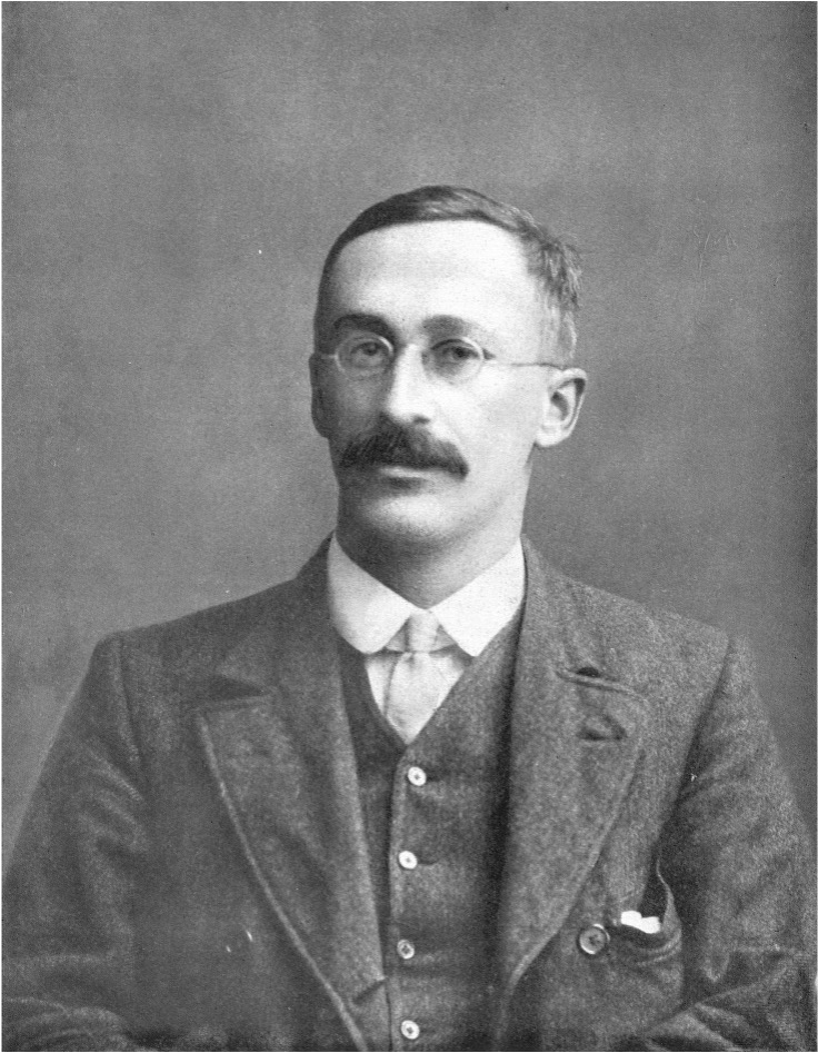
Fig. 9.8 William S. Gosset (1876-1937)

In 1908, William Sealy Gosset, a chemist and statistician employed by the Guinness brewery in Dublin, Ireland, published a paper titled “The Probable Error of a Mean” in the journal Biometrika. Due to Guinness company policy that prohibited employees from publishing their research, Gosset published under the pseudonym “Student”—leading to the now-famous Student’s t-distribution.

Gosset’s work at Guinness involved quality control for beer production. He needed statistical methods that worked reliably with small samples, as testing large quantities of beer would have been wasteful. Specifically, he faced the challenge of making inferences about a population mean when the population standard deviation was unknown and had to be estimated from the same limited sample.

His mathematical solution—the t-distribution—accounts for the added uncertainty of estimating \(\sigma\) with \(S\). This breakthrough has become one of the most widely used statistical tools across virtually all fields of scientific inquiry.

9.5.2. The t-Statistic and Its Distribution

To construct confidence regions, we have so far relied on the fact that the pivotal quantity \(\frac{\bar{X}-\mu}{\sigma/\sqrt{n}}\) follows a standard normal distribution under certain assumptions. When the unknown \(\sigma\) is replaced by its estimator \(S\), however, the resulting statistic

\[T_{n-1} = \frac{\bar{X} - \mu}{S/\sqrt{n}}\]

no longer follows a standard normal distribution. Instead, it follows a t-distribution.

The t-distribution is a family of continuous distributions parameterized by \(\nu\) (Greek letter “nu”; also called the degrees of freedom or df). A t-statistic constructed using a sample of size \(n\) has \(\nu = n-1\). The subscript in \(T_{n-1}\) reflects this fact, although it is often ommitted when the context makes it clear or when the detail is unnecessary.

Standardization, Studentization, and Pivotal Quantity

So far, we have called the transformation of a general random variable \(X\) into \(\frac{X-\mu_X}{\sigma_X}\) the standardization of \(X\). When the sample standard deviation \(S_X\) is used instead of \(\sigma_X\), giving

\[\frac{X-\mu_X}{S_X},\]

we call this the studentization of \(X\).

Both transformations are variants of pivotal quantities, which are functions of \(X\) constructed so that their distributions do not depend on the unkown parameters of \(X\).

Properties of t-Distributions

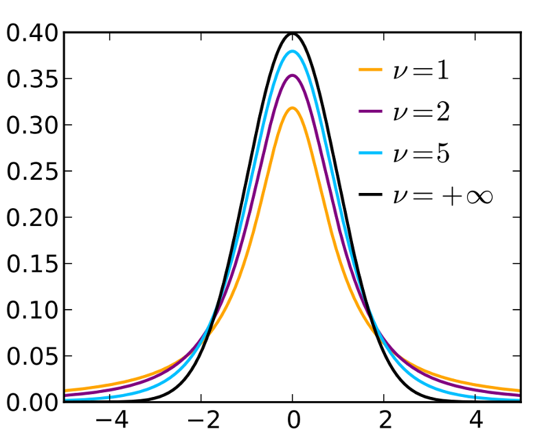
Fig. 9.9 t-densities with various degrees of freedom; the curve corresponding to \(+\infty\) is the standard normal PDF.

1. A t-distribution is symmetric around zero, similar to the standard normal distribution.

2. It has heavier tails than the standard normal distribution, reflecting the additional uncertainty from estimating \(\sigma\). This means that a t-distribution is always more spread out than the standard normal distribution for any finite degrees of freedom.

3. The smaller the sample size, the heavier the tails. The distribution approaches the standard normal distribution as the degrees of freedom increase.

The PDF of a t-distribution

The probability density function of a t-distribution is given by:

\[f_T(t) = \frac{1}{\sqrt{\nu\pi}} \frac{\Gamma(\frac{\nu+1}{2})}{\Gamma(\frac{\nu}{2})} \left(1 + \frac{t^2}{\nu}\right)^{-(\nu+1)/2}\]

Where \(\Gamma\), the gamma function, is a generalization of the factorial function. Just like normal distributions, we rely on tables or software to compute probabilities and percentiles involving t-distributions.

9.5.3. Deriving t-Based Confidence Regions

Preliminaries and Assumptions

The derivation of t-based confidence intervals requires a similar set of assumptions as before. The only difference is that \(\sigma\) is now unknown.

1. The data \(X_1, X_2, \cdots, X_n\) must be an iid sample from a population with mean \(\mu\) and variance \(\sigma^2.\)

2. Either the population is normally distributed, or we have sufficiently large \(n\) for the CLT to hold.

3. Both \(\mu\) and \(\sigma\) are unknown.

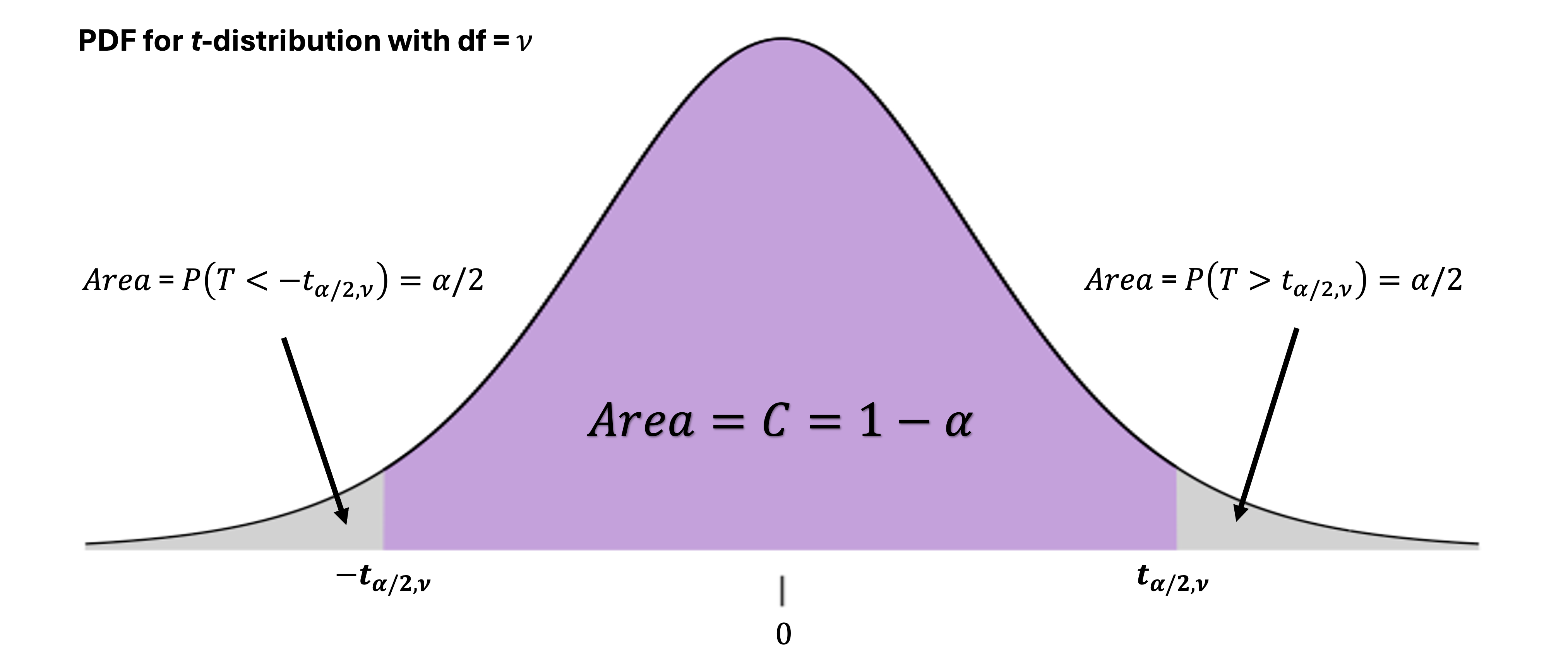
We also need to define the t-critical values. A t-critical value, denoted \(t_{\alpha/2, \nu}\), is the point on the t-distribution with \(\nu\) degrees of freedom such that its upper-tail area equals \(\alpha/2\). The notation includes an additional subscript for the degrees of freedom, since its location also depends on the specific t-distribution on which it is defined.

Derivation of the Confidence Interval

Similar to the case with known \(\sigma\), we derive a confidence interval for \(\mu\) using the pivotal method. For the degrees of freedom \(n-1\), the following statement is true by the definition of \(t_{\alpha/2, n-1}\):

\[P\left(-t_{\alpha/2, n-1} < T_{n-1} < t_{\alpha/2, n-1}\right) = C.\]

Replace \(T_{n-1}\) with the new pivotal quantity:

\[P\left(-t_{\alpha/2, n-1} < \frac{\bar{X} - \mu}{S/\sqrt{n}} < t_{\alpha/2, n-1}\right) = C.\]

Through algebraic pivoting, we isolate \(\mu\) to obtain:

\[P\left( \bar{X} - t_{\alpha/2, n-1} \frac{S}{\sqrt{n}}< \mu < \bar{X} + t_{\alpha/2, n-1} \frac{S}{\sqrt{n}}\right) = C.\]

Therefore, the \(C\cdot100\%\) confidence interval is:

\[\bar{X} \pm t_{\alpha/2, n-1} \frac{S}{\sqrt{n}}.\]

Summary of t-Based Confidence Intervals and Bounds

We leave it to the reader to work out the details of deriving the upper and lower confidence bounds under a t-distribution. The results follow the same pattern as their \(z\) equivalents; the margin of error will be computed with a smaller critical value \(t_{\alpha, n-1}\) instead of \(t_{\alpha/2, n-1}\).

In summary, when we have \(\bar{x}\) and \(s\) from an observed sample, we use the following formulas to compute confidence regions.

Confidence Regions When \(\sigma\) Is Unkonwn
Confidence Interval	\[\bar{x} \pm t_{\alpha/2, n-1} \frac{s}{\sqrt{n}}\]
Lower Confidence Bound	\[\bar{x} - t_{\alpha, n-1} \frac{s}{\sqrt{n}}\]
Upper Confidence Bound	\[\bar{x} + t_{\alpha, n-1} \frac{s}{\sqrt{n}}\]

Example 💡: Cholesterol Reduction Study

A pharmaceutical company is testing a new drug designed to lower LDL cholesterol levels. In a clinical trial, 15 patients with high cholesterol received the drug for eight weeks, and the reduction in their LDL cholesterol (in mg/dL) was measured.

The sample mean reduction was \(\bar{x} = 23.4\) mg/dL with a sample standard deviation of \(s = 6.8\) mg/dL. Construct a 95% confidence interval for the true mean reduction \(\mu\).

Step 1: Identify the key information

• Sample size: \(n = 15\)

• Sample mean: \(\bar{x} = 23.4\) mg/dL

• Sample standard deviation: \(s = 6.8\) mg/dL

• Confidence level: \(95\%\) (\(\alpha = 0.05\))

• Degrees of freedom: \(\nu = n - 1 = 14\)

Step 2: Find the critical value

\[t_{0.025, 14} = 2.145\]

qt(0.025, df = 14, lower.tail=FALSE)  # Returns 2.145

Step 3: Calculate the margin of error

\[\text{ME} = t_{0.025, 14} \cdot \frac{s}{\sqrt{n}} = 2.145 \cdot \frac{6.8}{\sqrt{15}} \approx 3.76 \text{ mg/dL}\]

Step 4: Construct the confidence interval

\[\bar{x} \pm \text{ME} = 23.4 \pm 3.76 = [19.64, 27.16] \text{ mg/dL}\]

Interpretation: We are 95% confident that the true mean reduction in LDL cholesterol with this drug is captured by the region between 19.64 and 27.16 mg/dL.

9.5.4. The Effect of Sample Size on t-Confidence Regions

As with \(z\)-confidence regions, a large \(n\) makes \(t\)-confidence regions more precise in general. However, the ways in which \(n\) influences this phenomenon are more multifaceted for t-based methods:

1. A larger \(n\) reduces the true standard error, \(\sigma/n\).

2. Although the true standard error is unknown, its estimator \(S/n\) targets it more accurately with larger \(n\).

3. The critical value itself decreases as \(n\) increases, which further narrows the confidence region.

To see how the third point holds, see Fig. 9.10 below:

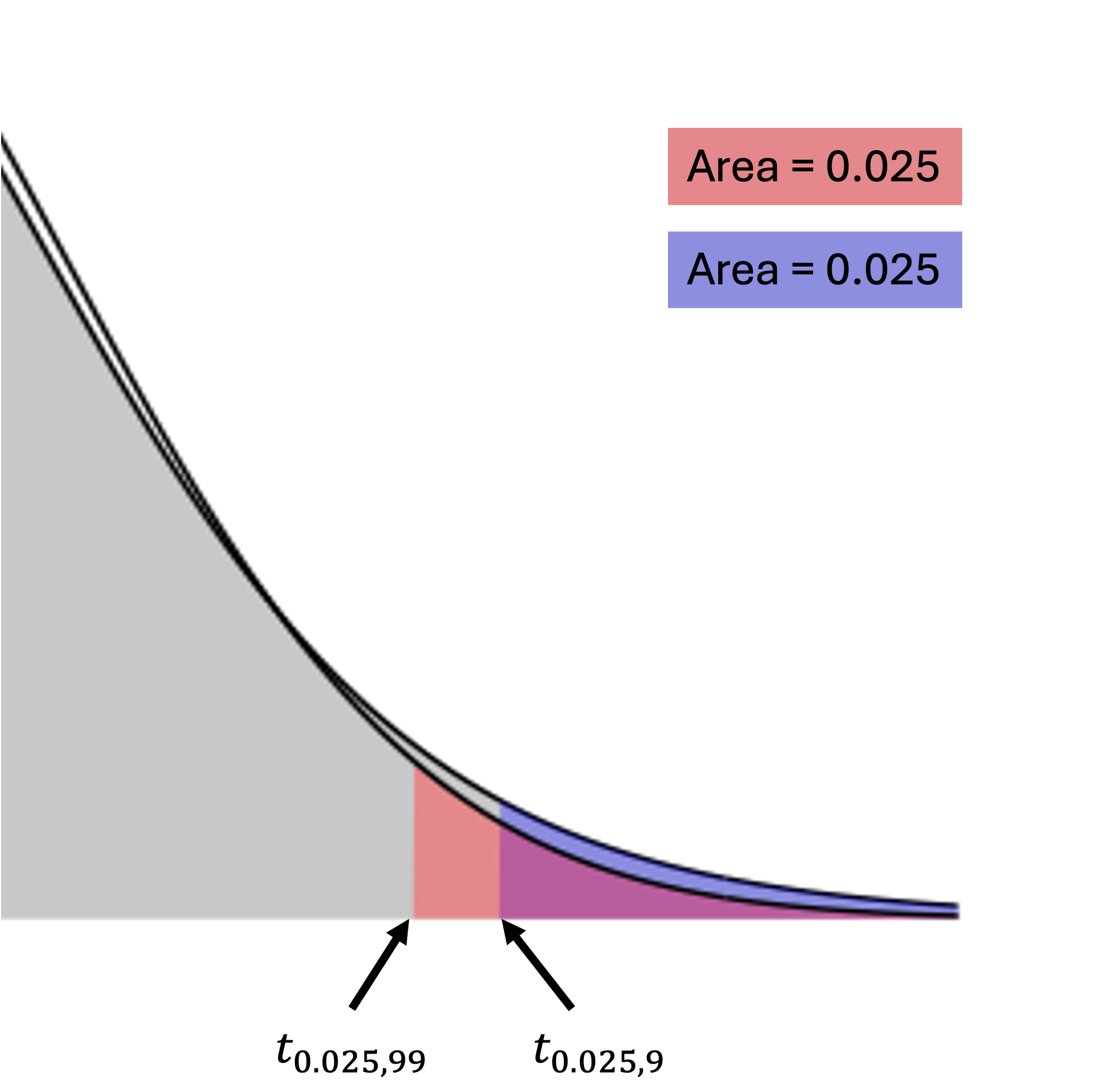
Fig. 9.10 Two-sided t-critical values for \(\alpha = 0.05\) with different degrees of freedom

In Fig. 9.10, the upper tails of two t-distributions are compared: one with \(df=n-1=99\) and the other with \(df=n-1=9\). Recall that higher degrees of freedom (and larger sample size) are associated with a lighter tail on a t-distribution. As \(n\) grows from 10 to 100, the difference in tail weight causes the critical value to move closer to the center (zero) in order to maintain an area of \(\alpha/2\) on its right.

In general, for the same confidence level and any two sample sizes \(n_1 < n_2\), it always holds that

\[t_{\alpha/2, n_1-1} > t_{\alpha/2, n_2-1}.\]

A smaller critical value leads to a smaller margin of error if \(s\) is held constant, which in turn results in a more precise (narrower) confidence region. This relationship does not hold strictly in practice since \(S\) fluctuates with data, but the overall tendency remains.

Comparison with \(z\)-Confidence Regions

The above result implies that the \(z\)-confidence regions— which can loosely be considered t-confidence regions with an “infinite” dataset for sample variance computation—are more precise on average than their t-based parallels.

When is a \(t\)-Confidence Region Appropriate?

In practice, the true variance \(\sigma^2\) is rarely known, leaving t-procedures as our only option. On the rare occasions when \(\sigma^2\) is known, it is always preferabale to use this true information.

9.5.5. Sample Size Planning When σ Is Unknown

Sample size planning is more challenging when \(\sigma\) is unknown. Suppose we want \(n\) such that

\[\text{ME} = t_{\alpha/2, n-1} \frac{s}{\sqrt{n}} \leq ME_{max}\]

for some given maximum margin of error, \(ME_{max}\). By taking similar steps as in Chapter 9.3.2, we have

\[n \geq \left(\frac{t_{\alpha/2, n-1}s}{ME_{max}}\right)^2.\]

We now see that the problem is circular. To determine \(n\), we need the \(t\)-critical value, which depends on \(n\). Additionally, we need a value for \(s\), which we don’t have before collecting data. To address this issue, we use an iterative approach involving the following steps:

1. Obtain a planning value \(s_*\). This can be done by

   • Using \(s\) from a pilot study or previous research,

   • Making an educated guess based on the expected range, or

   • Using a conservative upper bound when uncertainty is high.

2. Update \(n\) iteratively.

   • Start with an initial guess using the \(z\)-critical value: \(n_0 = \left(\frac{z_{\alpha/2} s_*}{ME_{max}}\right)^2\).

   • Calculate the t-critical value using \(df = n_0 - 1\).

   • Recalculate \(n\) using the t-critical value.

   • Repeat until convergence.

This process typically converges quickly, often in just a few iterations.

9.5.6. Robustness of the \(t\)-Procedures

A statistical procedure is considered robust if it performs reasonably well even when its assumptions are somewhat violated. The \(t\)-procedures show good robustness against moderate departures from normality, especially as sample size increases.

Guidelines for Using t-Procedures When Normality May Not Hold
\(n < 15\)	The population distribution should be approximately normal. Check the sample data with normal probability plots.
\(15 ≤ n < 40\)	A \(t\)-procedure works well with some mild skewness. Avoid using with strongly skewed data or data containing outliers.
\(n ≥ 40\)	A \(t\)-procedure is generally reliable even with moderately skewed distributions, thanks to the Central Limit Theorem.

Regardless of sample size, the procedure is sensitive to outliers, which can strongly influence both \(\bar{x}\) and \(s\). Always inspect your data for outliers before applying a \(t\)-procedure.

9.5.7. Bringing It All Together

Key Takeaways 📝

• The Student’s t-distribution provides the appropriate framework for quantifying uncertainty about a population mean when the population standard deviation is unknown.

• The pivotal quantity \(T_{n-1}= \frac{\bar{X}-\mu}{S/\sqrt{n}}\) now follows a t-distribution with \(n-1\) degrees of freedom.

• The resulting confidence regions account for the additional uncertainty in estimating \(\sigma\), and are wider than their \(z\) parallels on average.

• The t-procedures are robust to moderate violations of the normality assumption. The robustness grows with the sample size.

Exercises

1. A quality control engineer wants to estimate the mean tensile strength of steel cables. A sample of 25 cables yields a mean strength of 3450 N with a standard deviation of 120 N. Construct a 99% confidence interval for the mean strength.

2. A pilot study with 8 observations yielded a sample standard deviation of \(s = 15\). If a researcher wants to estimate the population mean with a margin of error of no more than 5 units at 95% confidence, how many observations should be planned for the full study?

Exercises: CI and Confidence Bounds (σ Unknown)

Learning Objectives 🎯

These exercises will help you:

• Recognize when to use the t-distribution instead of the z-distribution

• Find t-critical values for various confidence levels and degrees of freedom

• Construct confidence intervals for μ when σ is unknown

• Construct confidence bounds (UCB/LCB) when σ is unknown

• Understand the relationship between t and z as df increases

• Assess robustness of t-procedures to non-normality

Key Formulas 📐

Confidence Interval for μ (σ unknown):

\[\bar{x} \pm t_{\alpha/2, n-1} \frac{s}{\sqrt{n}}\]

Confidence Bounds (σ unknown):

\[UCB = \bar{x} + t_{\alpha, n-1} \frac{s}{\sqrt{n}} \qquad LCB = \bar{x} - t_{\alpha, n-1} \frac{s}{\sqrt{n}}\]

Degrees of freedom: \(df = n - 1\)

R Functions:

# t-critical values
qt(alpha/2, df, lower.tail = FALSE)  # For CI
qt(alpha, df, lower.tail = FALSE)    # For bounds

# One-sample t-test with CI
t.test(x, conf.level = 0.95)

9.5.8. Exercises

Exercise 1: t-Distribution Properties

1. When do we use the t-distribution instead of the z-distribution for inference about μ?

2. What are the degrees of freedom for a one-sample t-procedure with sample size n?

3. How does the shape of the t-distribution compare to the standard normal? What causes this difference?

4. As degrees of freedom increase, what happens to the t-distribution?

5. Find \(t_{0.025, 15}\) and \(z_{0.025}\). Which is larger? Why?

Solution

Part (a): When to use t-distribution

Use the t-distribution when:

• Making inference about the population mean μ

• The population standard deviation σ is unknown and must be estimated by s

• The underlying population is approximately normal (or n is large enough for CLT)

Part (b): Degrees of freedom

For a one-sample t-procedure: \(df = n - 1\)

Part (c): Shape comparison

The t-distribution is:

• Symmetric and bell-shaped like the normal

• Heavier tails than the standard normal (more probability in the extremes)

• This occurs because using s instead of σ introduces additional uncertainty

Part (d): As df increases

As df → ∞, the t-distribution approaches the standard normal distribution.

Rule of thumb: By df ≈ 30, t-critical values are close to z-critical values for most practical purposes. By df ≈ 100, the difference is negligible.

Part (e): Comparing critical values

qt(0.025, 15, lower.tail = FALSE)  # 2.131
qnorm(0.025, lower.tail = FALSE)   # 1.960

\(t_{0.025, 15} = 2.131 > z_{0.025} = 1.960\)

The t-critical value is larger because the heavier tails of the t-distribution require going further from the center to capture 97.5% of the probability.

---

Exercise 2: Finding t-Critical Values

Find the t-critical value for each scenario using R or a t-table.

1. 95% CI, n = 10

2. 95% CI, n = 25

3. 99% CI, n = 20

4. 90% UCB, n = 15

5. 95% LCB, n = 30

6. 95% CI, n = 200 (compare to z-critical value)

Solution

Part (a): 95% CI, n = 10 (df = 9)

\(t_{0.025, 9} = 2.262\)

Part (b): 95% CI, n = 25 (df = 24)

\(t_{0.025, 24} = 2.064\)

Part (c): 99% CI, n = 20 (df = 19)

\(t_{0.005, 19} = 2.861\)

Part (d): 90% UCB, n = 15 (df = 14)

\(t_{0.10, 14} = 1.345\)

Part (e): 95% LCB, n = 30 (df = 29)

\(t_{0.05, 29} = 1.699\)

Part (f): 95% CI, n = 200 (df = 199)

\(t_{0.025, 199} = 1.972\) vs \(z_{0.025} = 1.960\)

Difference is only 0.012—practically identical.

R verification:

qt(0.025, 9, lower.tail = FALSE)    # 2.262
qt(0.025, 24, lower.tail = FALSE)   # 2.064
qt(0.005, 19, lower.tail = FALSE)   # 2.861
qt(0.10, 14, lower.tail = FALSE)    # 1.345
qt(0.05, 29, lower.tail = FALSE)    # 1.699
qt(0.025, 199, lower.tail = FALSE)  # 1.972

---

Exercise 3: Basic CI Construction (σ Unknown)

A chemical engineer measures the purity of a batch of pharmaceutical product. A random sample of n = 12 measurements yields:

• Sample mean: \(\bar{x} = 98.45\%\)

• Sample standard deviation: \(s = 1.23\%\)

1. Find the appropriate t-critical value for a 95% CI.

2. Calculate the estimated standard error.

3. Calculate the margin of error.

4. Construct the 95% confidence interval.

5. Interpret the interval in context.

Solution

Given: n = 12, \(\bar{x} = 98.45\%\), s = 1.23%

Part (a): t-critical value

df = 12 - 1 = 11

\(t_{0.025, 11} = 2.201\)

Part (b): Estimated standard error

\[\widehat{SE} = \frac{s}{\sqrt{n}} = \frac{1.23}{\sqrt{12}} = 0.355\%\]

Part (c): Margin of error

\[ME = t_{0.025, 11} \times \widehat{SE} = 2.201 \times 0.355 = 0.781\%\]

Part (d): 95% CI

\[CI: 98.45 \pm 0.78 = (97.67\%, 99.23\%)\]

Part (e): Interpretation

We are 95% confident that the true mean purity of this pharmaceutical batch is between 97.67% and 99.23%.

R verification:

xbar <- 98.45; s <- 1.23; n <- 12
df <- n - 1
t_crit <- qt(0.025, df, lower.tail = FALSE)
SE <- s / sqrt(n)
ME <- t_crit * SE
c(xbar - ME, xbar + ME)  # [97.67, 99.23]

---

Exercise 4: CI from Raw Data

A biomedical engineer tests the glucose response time (seconds) of a new blood glucose monitor. The measured times from 8 test samples are:

4.2, 3.8, 4.5, 4.1, 3.9, 4.4, 4.0, 4.3

1. Calculate \(\bar{x}\) and \(s\).

2. Construct a 95% confidence interval for the mean response time.

3. The manufacturer claims the mean response time is 4.0 seconds. Is this claim consistent with your interval?

4. Use R’s t.test() function to verify your results.

Solution

Part (a): Summary statistics

times <- c(4.2, 3.8, 4.5, 4.1, 3.9, 4.4, 4.0, 4.3)
mean(times)  # 4.15
sd(times)    # 0.2449

\(\bar{x} = 4.15\) seconds, \(s = 0.245\) seconds

Part (b): 95% CI

n = 8, df = 7

\(t_{0.025, 7} = 2.365\)

\[\widehat{SE} = \frac{0.245}{\sqrt{8}} = 0.0866\]

\[ME = 2.365 \times 0.0866 = 0.205\]

\[CI: 4.15 \pm 0.205 = (3.95, 4.35) \text{ seconds}\]

Part (c): Manufacturer’s claim

The claimed value of 4.0 seconds is within the 95% CI (3.95, 4.35). Yes, the claim is consistent with the data.

Part (d): R verification

times <- c(4.2, 3.8, 4.5, 4.1, 3.9, 4.4, 4.0, 4.3)
t.test(times, conf.level = 0.95)

# Output includes:
# 95 percent confidence interval:
#  3.945 to 4.355
# sample mean: 4.15

---

Exercise 5: Confidence Bounds (σ Unknown)

A quality engineer tests the breaking strength (in Newtons) of climbing rope. From n = 15 samples:

• \(\bar{x} = 2850\) N

• \(s = 125\) N

1. Construct a 95% lower confidence bound for mean breaking strength.

2. Safety standards require mean strength of at least 2700 N. Does the rope meet this standard?

3. Construct a 95% upper confidence bound.

4. Compare the bounds to a 95% two-sided CI. Which provides tighter information about each limit?

Solution

Given: n = 15, \(\bar{x} = 2850\) N, s = 125 N, df = 14

\(\widehat{SE} = \frac{125}{\sqrt{15}} = 32.27\) N

Part (a): 95% LCB

\(t_{0.05, 14} = 1.761\)

\[LCB = 2850 - 1.761 \times 32.27 = 2850 - 56.8 = 2793.2 \text{ N}\]

Part (b): Safety standard

LCB (2793.2 N) > 2700 N requirement. Yes, the rope meets the safety standard with 95% confidence.

Part (c): 95% UCB

\[UCB = 2850 + 1.761 \times 32.27 = 2850 + 56.8 = 2906.8 \text{ N}\]

Part (d): Comparison to CI

95% CI using \(t_{0.025, 14} = 2.145\):

\[ME = 2.145 \times 32.27 = 69.2 \text{ N}\]

\[CI: (2780.8, 2919.2) \text{ N}\]

Comparison:

• CI lower bound: 2780.8 N; LCB: 2793.2 N (LCB is tighter/higher)

• CI upper bound: 2919.2 N; UCB: 2906.8 N (UCB is tighter/lower)

One-sided bounds provide tighter limits on the side of interest because they use \(t_{\alpha}\) instead of \(t_{\alpha/2}\), and \(t_{0.05} < t_{0.025}\). The UCB is tighter than the CI’s upper bound; the LCB is tighter than the CI’s lower bound.

---

Exercise 6: Comparing z and t Intervals

A sensor is tested with n = 20 measurements: \(\bar{x} = 152.3\) units, \(s = 8.4\) units. Compare:

1. Compute a 95% CI using the t-distribution (correct method).

2. Compute what the CI would be if you incorrectly used the z-distribution with s.

3. Which interval is wider? Why is using z inappropriate here?

4. At what sample size would the difference become negligible?

Solution

Given: n = 20, \(\bar{x} = 152.3\), s = 8.4, df = 19

\(\widehat{SE} = \frac{8.4}{\sqrt{20}} = 1.878\)

Part (a): Correct t-interval

\(t_{0.025, 19} = 2.093\)

\[CI: 152.3 \pm 2.093 \times 1.878 = 152.3 \pm 3.93 = (148.37, 156.23)\]

Part (b): Incorrect z-interval

\(z_{0.025} = 1.96\)

\[CI: 152.3 \pm 1.96 \times 1.878 = 152.3 \pm 3.68 = (148.62, 155.98)\]

Part (c): Comparison

The t-interval (width = 7.86) is wider than the z-interval (width = 7.36).

Using z is inappropriate because:

• σ is unknown and estimated by s

• Using s introduces additional variability not accounted for by z

• The t-distribution properly inflates the critical value to compensate

Part (d): When difference becomes negligible

For df ≈ 30, \(t_{0.025, 30} = 2.042\) vs \(z_{0.025} = 1.96\) (difference ≈ 4%)

For df ≈ 100, \(t_{0.025, 100} = 1.984\) vs \(z_{0.025} = 1.96\) (difference ≈ 1%)

For most practical purposes, the difference is negligible when n > 100 or so.

---

Exercise 7: Multiple Confidence Levels

Using the data from Exercise 3 (n = 12, \(\bar{x} = 98.45\%\), s = 1.23%):

1. Construct 90%, 95%, and 99% confidence intervals.

2. Create a table showing confidence level, t-critical value, ME, and interval bounds.

3. What pattern do you observe?

4. If the specification requires purity above 97.5%, at which confidence level(s) can you confidently claim compliance?

Solution

Given: n = 12, df = 11, \(\bar{x} = 98.45\%\), s = 1.23%, \(\widehat{SE} = 0.355\%\)

Parts (a) and (b): Table

Confidence	\(t_{crit}\)	ME	Lower	Upper
90%	1.796	0.638	97.81	99.09
95%	2.201	0.781	97.67	99.23
99%	3.106	1.103	97.35	99.55

Part (c): Pattern

As confidence level increases:

• t-critical value increases

• Margin of error increases

• Interval width increases

Higher confidence requires wider intervals.

Part (d): Compliance claim

Specification: purity > 97.5%

• At 90%: Lower bound (97.81) > 97.5 ✓

• At 95%: Lower bound (97.67) > 97.5 ✓

• At 99%: Lower bound (97.35) < 97.5 ✗

Can claim compliance at 90% and 95% confidence, but not at 99%.

R verification:

xbar <- 98.45; s <- 1.23; n <- 12
SE <- s / sqrt(n)

conf_levels <- c(0.90, 0.95, 0.99)
alpha <- 1 - conf_levels
t_crits <- qt(alpha/2, df = 11, lower.tail = FALSE)
MEs <- t_crits * SE

data.frame(
  Confidence = paste0(conf_levels * 100, "%"),
  t_crit = round(t_crits, 3),
  ME = round(MEs, 3),
  Lower = round(xbar - MEs, 2),
  Upper = round(xbar + MEs, 2)
)

---

Exercise 8: Robustness to Non-Normality

The t-procedures assume the population is approximately normal. However, they are somewhat robust to departures from normality.

1. For what sample sizes are t-procedures most sensitive to non-normality?

2. What features of a distribution are most problematic for t-procedures?

3. Given a sample with n = 8 that contains one apparent outlier, what should you do before constructing a CI?

4. A researcher has n = 50 observations from a mildly skewed population. Is it appropriate to use t-procedures?

5. If you discover a problematic outlier after constructing a CI, what remedies might you consider?

Solution

Part (a): Most sensitive sample sizes

t-procedures are most sensitive to non-normality when n is small (generally n < 15). With small samples, there’s little averaging to invoke the CLT, so the normality assumption is more critical.

Guidelines:

• n < 15: Population should be approximately normal with no outliers. t-procedures are sensitive to non-normality at small sample sizes.

• 15 ≤ n < 30: Mild departures from normality are acceptable; avoid strong skewness or outliers

• n ≥ 30: t-procedures are reasonably robust; even moderately skewed populations are okay

• n ≥ 50: Very robust to non-normality due to CLT

Part (b): Problematic distribution features

• Outliers: Most problematic—inflate s and distort \(\bar{x}\)

• Strong skewness: Asymmetry can bias the sample mean

• Heavy tails: Increase the chance of extreme observations

• Bimodality: Violates the single-peak assumption

Part (c): Outlier in small sample (n = 8)

Before constructing a CI:

1. Investigate the outlier—is it a measurement error, data entry error, or legitimate observation?

2. Create diagnostic plots (histogram, boxplot, QQ-plot)

3. If error: correct or remove with justification

4. If legitimate: consider the impact on results; report both with and without the outlier

5. Consider robust alternatives if available

Part (d): n = 50, mildly skewed

Yes, appropriate. With n = 50, the CLT ensures the sampling distribution of \(\bar{x}\) is approximately normal even if the population is mildly skewed. t-procedures are robust at this sample size.

Part (e): Remedies for problematic outliers

If an outlier is discovered after constructing a CI:

1. Investigate: Determine if it’s an error or valid data point

2. Consider removal: If there’s justification (measurement error, data recording mistake), remove and recompute

3. Acknowledge robust alternatives: Median-based CI or bootstrap methods (not covered in this course) are less sensitive to outliers

4. Report with caution: If the outlier appears valid, interpret results carefully and note the limitation

---

Exercise 9: Sample Size Planning with Unknown σ

When planning sample size with σ unknown, we face a challenge: we need s to find the t-critical value, but we don’t have data yet.

A researcher wants a 95% CI for mean reaction time with ME ≤ 5 ms. A pilot study suggests s ≈ 20 ms.

1. Using the z-approximation (pretending σ = 20), calculate the required sample size.

2. Using the result from (a), find \(t_{0.025, n-1}\) and recalculate the required n.

3. Iterate: with the new n, find the new t-critical value and check if n is sufficient.

4. What is the final recommended sample size?

Solution

Given: 95% CI, ME ≤ 5 ms, estimated s = 20 ms

Step 1 — Initial z-approximation

\[n = \left\lceil \left(\frac{1.96 \times 20}{5}\right)^2 \right\rceil = \left\lceil 61.47 \right\rceil = 62\]

Step 2 — First iteration with t

With n = 62, df = 61: \(t_{0.025, 61} = 2.000\)

\[n = \left\lceil \left(\frac{2.000 \times 20}{5}\right)^2 \right\rceil = \left\lceil 64 \right\rceil = 64\]

Step 3 — Check for convergence

With n = 64, df = 63: \(t_{0.025, 63} = 1.998\)

\[n = \left\lceil \left(\frac{1.998 \times 20}{5}\right)^2 \right\rceil = \left\lceil 63.87 \right\rceil = 64\]

Converged!

Part (d): Final recommendation

n = 64 samples

Note: One or two iterations is typically sufficient because t-critical values change slowly once df is moderate (beyond about 20).

R verification:

s <- 20; ME <- 5

# Initial z-approximation
n1 <- ceiling((qnorm(0.025, lower.tail=FALSE) * s / ME)^2)  # 62

# First iteration
n2 <- ceiling((qt(0.025, n1-1, lower.tail=FALSE) * s / ME)^2)  # 64

# Second iteration
n3 <- ceiling((qt(0.025, n2-1, lower.tail=FALSE) * s / ME)^2)  # 64

# Verify
qt(0.025, 63, lower.tail = FALSE)  # 1.998

---

9.5.9. Additional Practice Problems

True/False Questions (1 point each)

1. The t-distribution has heavier tails than the standard normal distribution.

   Ⓣ or Ⓕ

2. As degrees of freedom increase, t-critical values approach z-critical values.

   Ⓣ or Ⓕ

3. For a one-sample t-procedure with n = 20, the degrees of freedom is 20.

   Ⓣ or Ⓕ

4. The t-distribution is appropriate when σ is known.

   Ⓣ or Ⓕ

5. A 95% CI using t will always be wider than one using z (same data).

   Ⓣ or Ⓕ

6. t-procedures require the population to be exactly normal.

   Ⓣ or Ⓕ

Multiple Choice Questions (2 points each)

7. For n = 25 and 95% confidence, the appropriate critical value is:

   Ⓐ \(z_{0.025} = 1.96\)

   Ⓑ \(t_{0.025, 25} = 2.060\)

   Ⓒ \(t_{0.025, 24} = 2.064\)

   Ⓓ \(t_{0.05, 24} = 1.711\)

8. If \(\bar{x} = 45\), s = 6, n = 16, the 95% CI is approximately:

   Ⓐ 45 ± 2.131(1.5)

   Ⓑ 45 ± 1.96(1.5)

   Ⓒ 45 ± 2.131(6)

   Ⓓ 45 ± 1.753(1.5)

9. The degrees of freedom for a one-sample t-test equals n - 1 because:

   Ⓐ One observation is lost to rounding

   Ⓑ We estimate one parameter (μ) from the data

   Ⓒ We estimate one parameter (σ) using s, losing one degree of freedom

   Ⓓ The sample size must be reduced by 1

10. t-procedures are most robust to non-normality when:

    Ⓐ Sample size is very small (n < 10)

    Ⓑ Sample size is moderate to large (n ≥ 30)

    Ⓒ The population is heavily skewed

    Ⓓ Outliers are present

11. For a 90% LCB with n = 20, the critical value is:

    Ⓐ \(t_{0.10, 19}\)

    Ⓑ \(t_{0.05, 19}\)

    Ⓒ \(t_{0.10, 20}\)

    Ⓓ \(z_{0.10}\)

12. Which R command gives a 95% CI for mean of vector x?

    Ⓐ t.test(x)

    Ⓑ z.test(x)

    Ⓒ confint(x)

    Ⓓ qt(0.025, length(x))

Answers to Practice Problems

True/False Answers:

1. True — The t-distribution has heavier tails to account for uncertainty in estimating σ.

2. True — As df → ∞, t → z. By df ≈ 30, they’re close; by df ≈ 100, nearly identical.

3. False — df = n - 1 = 19, not 20.

4. False — When σ is known, use the z-distribution. t is for σ unknown.

5. True — t-critical values exceed z-critical values for all finite df.

6. False — t-procedures are robust to mild departures, especially with larger samples.

Multiple Choice Answers:

7. Ⓒ — df = n - 1 = 24, and for a CI use \(t_{0.025, 24}\).

8. Ⓐ — SE = 6/√16 = 1.5; df = 15; \(t_{0.025, 15} = 2.131\).

9. Ⓒ — We use one degree of freedom to estimate σ with s.

10. Ⓑ — Larger samples invoke CLT, making the procedure robust to non-normality.

11. Ⓐ — For a one-sided bound at 90% confidence, use \(t_{0.10, n-1} = t_{0.10, 19}\).

12. Ⓐ — t.test(x) computes the one-sample t-test and 95% CI by default.