Slides 📊

• Hypothesis Testing for Single Sample (Part 4) (PPTX)

10.4. The Four Steps to Hypothesis Testing and Understanding the Result

We conclude our introduction to hypothesis testing by stepping back to examine the broader picture. We present a standardized four-step framework to hypothesis testing and discuss important subtleties in its interpretation. In particular, we address what hypothesis tests can and cannot tell us, how to interpret results responsibly, and common pitfalls to avoid in practice.

Road Map 🧭

• Organize the hypothesis testing workflow into four steps: (1) define the parameter(s), (2) state the hypotheses, (3) compute the test statistic, the df, and the \(p\)-value, (4) draw a conclusion.

• Correctly interpret \(p\)-values and statistically significant results.

• Recognize ethical and practical concerns regarding statistical inference.

10.4.1. The Four-Step Process to Hypothesis Testing

Throughout our exploration of hypothesis testing, we have been following an implicit structure. Now let us formalize this into a systematic four-step process that ensures consistency and completeness in our analysis.

Step 1: Identify and Describe the Parameter(s) of Interest

Make a concrete connection between the context of the problem and the mathematical notation to be used in the formal test. This step should include:

• The population being studied

• The symbol for the parameter of interest (e.g., \(\mu\))

• What the parameter represents in practical terms

• Units of measurement

• Any other contextual details needed for interpretation

Example 💡: Testing Water Recycling Performance–Step 1

The Whimsical Wet ‘n’ Wobble Water Wonderland Waterpark has implemented a new water recycling system. This recycling system is supposed to ensure water loss only due to evaporation and splashing by the park patrons. However, after its implementation, they suspect a higher daily water loss than the pre-implementation average of 230,000 gallons per day.

To investigate, the park collected 21 days of water usage data during the first year of implementation. Perform a hypothesis test to determine if the system underperforms expectations. Use a \(\alpha=0.05\) significance level.

Step 1 of the Hypothesis Test

Let \(\mu\) represent the true average daily water loss (in thousands of gallons) at the Whimsical Wet ‘n’ Wobble Water Wonderland Waterpark after implementing the new recycling system.

Step 2: State the Hypotheses

State the paired hypotheses in the correct mathematical format. Refer to the rules listed in Chapter 10.1.1.

Example 💡: Testing Water Recycling Performance–Step 2

Continuing from the context provided in the previous example,

Step 2 of the Hypothesis Test

\[\begin{split}&H_0: \mu \leq 230\\ &H_a: \mu > 230\end{split}\]

Step 3: Calculate the Test Statistic and P-Value

Perform all the computational steps. This includes:

• Checking that the normality assumption is reasonably met

• Deciding between a \(z\)-test or a \(t\)-test based on whether the population standard deviation is known

• Computing the test statistic and stating the appropriate degrees of freedom, if any

• Calculating the \(p\)-value

Example 💡: Testing Water Recycling Performance–Step 3

The 21 daily water loss measurements, in thousands of gallons, are:

190.1	244.6	244.1	270.1	269.6	201.0	234.3
292.3	205.7	242.3	263.0	219.0	233.3	229.0
293.5	290.4	264.0	248.6	260.5	210.4	236.9

Step 3 of the Hypothesis Test

Graphical analysis of the data’s distribution:

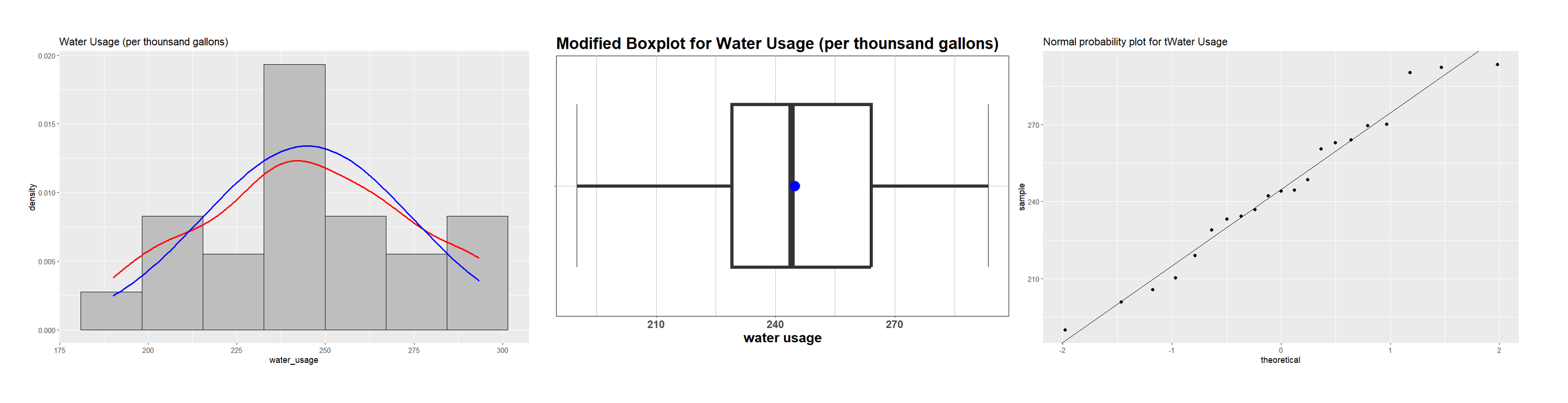
Fig. 10.29 Graphical assessment of normality

The data distribution shows moderate deviation from normality, for which the sample size of \(n=21\) is large enough. In addition, the population standard deviation is unknown. Therefore, we use the \(t\)-test procedure.

The numerical summaries:

• \(n=21\)

• \(\bar{x} = 244.8905\)

• \(s=29.81\)

• \(df = n-1 = 20\)

The observed test statistic:

\[t_{TS} = \frac{244.8905-230}{29.81/\sqrt{n}} = 2.2891\]

The \(p\)-value:

\[p = P(T_{n-1} > t_{TS}) = P(T_{20} > 2.2891) = 0.01654,\]

which can be computed using the R code below:

pvalue <- pt(2.2891, df=20, lower.tail=FALSE)

Step 4: Make the Decision and State the Conclusion

This step consists of two parts.

First, draw a formal decision: compare the \(p\)-value computed in Step 3 to \(\alpha\) and state whether the null hypothes is is rejected. We never “reject the alternative” or “accept” anything. The only two choices available for a formal decision is to

• reject the null hypothesis, or

• fail to reject the null hypothesis.

Then make a contextual conclusion using the template below:

“The data [does/does not] give [some/strong] support (p-value = [actual value]) to the claim that [statement of \(H_a\) in context].”

Example 💡: Testing Water Recycling Performance–Step 4

The waterpark required the test to have the significance level \(\alpha=0.05\).

Step 4 of Hypothesis Testing

Since \(p\)-value \(= 0.01654 < 0.05\), the null hypothesis is rejected. There is sufficient evidence from data (\(p\)-value \(= 0.01654\)) to the claim that the true mean daily water loss after implementing the new water recycling system is greater than 230,000 gallons.

10.4.2. Understanding Statistical Significance

We call a statistical result whose behavior may be attributed to more than just random chance statistically significant. In hypothesis testing, results that lead to rejection of the null hypothesis are conventionally regarded as statistically significant.

However, when we encounter a \(p\)-value smaller than \(\alpha\) in practice, the information conveyed can be more nuanced than it may first appear. A statistically significant result can arise to a combination of the following three reasons:

1. Existence of True Effect (What We Hope For)

We may encounter a statistically significant result because the null hypothesis is actually false and our test correctly identified a genuine effect. This represents the ideal scenario where statistical significance corresponds to a real phenomenon.

2. Rare Event Under True Null

Even if the null hypothesis is true, we could observe extreme data purely by chance. Our significance level \(\alpha\) represents our tolerance for this type of error (Type I error). If \(\alpha = 0.05\), we expect to falsely reject true null hypotheses about 5% of the time in the long run.

3. Assumption Violations

Hypothesis tests rely on assumptions about the population and the sampling procedure. The data can be flagged as unusual by a hyopothesis test when the background assumptions are incorrect.

The Key Message

A statistically significant result indicates inconsistency between the data and the assumptions. For the result to be meaningful, we must ensure that the only assumption that can be violated is the null hypothesis. This is why checking the distributional assumptions thoroughly before inference is essential.

10.4.3. What \(p\)-Values Are and What They Are Not

Recall that a \(p\)-value is the probability of obtaining a test statistic at least as extreme as the one observed, assuming the null hypothesis and all other model assumptions are true. It quantifies how incompatible the data are with the null hypothesis.

What \(p\)-Values Are NOT

❌ The p-value is NOT the probability that the null hypothesis is true.

A \(p\)-value of 0.03 does not mean there’s a 3% chance the null hypothesis is correct.

❌ The p-value is NOT the probability that observations occurred by chance.

The \(p\)-value is computed under the assumption that the null hypothesis and all model assumptions are true. It’s the probability of the data given these assumptions, not the probability that chance alone explains the results.

❌ A small p-value does NOT prove the null hypothesis false.

A small \(p\)-value flags the data as unusual under our assumptions. This could mean that:

• The null hypothesis is false (what we hope).

• A rare event occurred under a true null hypothesis.

• Model assumptions are violated.

❌ A large p-value does NOT prove the null hypothesis true

A large \(p\)-value simply indicates that the data is consistent with the null hypothesis. This could mean that:

• The null hypothesis is actually true.

• Our sample size was too small to detect an existing effect.

• The effect size is too small to detect with our current design.

10.4.4. The Problem of \(p\)-Value Hacking

Unfortunately, the pressure to publish statistically significant results has led to unethical practices collectively known as \(p\)-value hacking, data dredging, or fishing for significance.

Common Forms of \(p\)-Value Hacking

• Conducting multiple analyses but selectively reporting only those yielding significant results.

• Data Manipulation, such as increasing the data size until reaching significance, excluding problematic observations, and trying different response variables until finding a significant one

• Model Shopping, or trying different statistical procedures until finding one that yields significance, without proper justification for the model choice.

Preventing \(p\)-Value Hacking

\(p\)-value hacking leads to increased false positives, undermining confidence in research findings. Forgood research practice, a researcher should:

• document all procedures, including any data exclusions,

• report all analyses conducted, not just significant ones, and

• specify hypotheses and analysis plans before data collection.

10.4.5. Bringing It All Together

Key Takeaways 📝

1. Organize your hypothesis testing workflow in four steps:

   1. parameter identification,

   2. hypothesis statement,

   3. calculation, and

   4. decision and conclusion in context.

2. Know the correct implications of statistical significance and \(p\)-values.

3. \(p\)-value hacking undermines scientific integrity. For good research practice, determine the complete analysis plan prior to data collection and document all procedures transparently.

10.4.6. Exercises

Exercise 1: Correct P-value Interpretation

For each statement about a p-value of 0.03, indicate whether it is CORRECT or INCORRECT. Explain why.

1. “There is a 3% probability that the null hypothesis is true.”

2. “If the null hypothesis is true, there is a 3% probability of observing data at least as extreme as what we obtained.”

3. “There is a 3% probability that our results occurred by random chance.”

4. “The probability of a Type I error is 3%.”

5. “We have proven that the alternative hypothesis is true with 97% confidence.”

6. “If we repeated this study many times when H₀ is true, about 3% of the studies would yield a test statistic this extreme or more.”

Solution

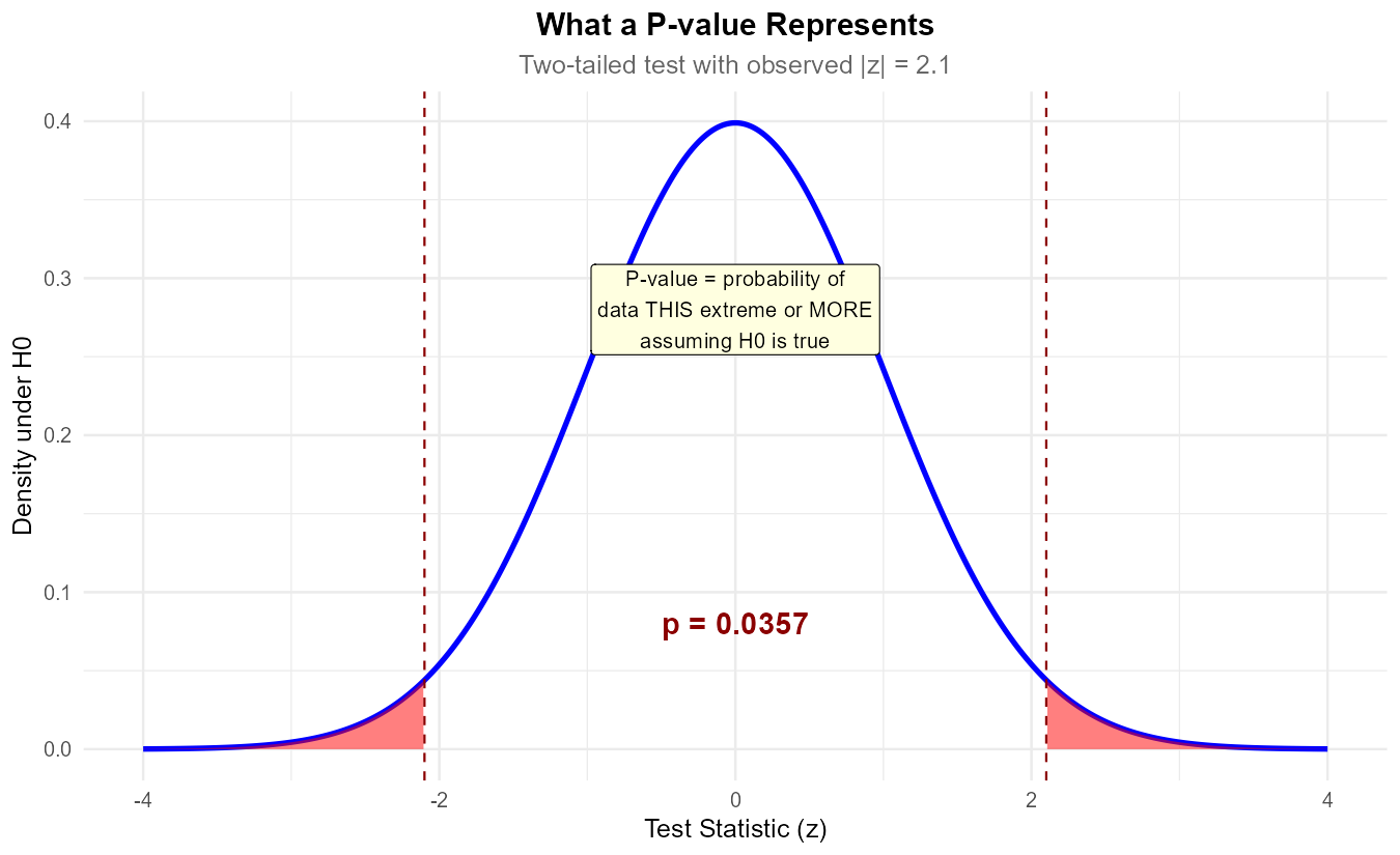
Fig. 10.30 The p-value is the probability of data this extreme or more extreme, assuming H₀ is true.

Part (a): INCORRECT ✗

The p-value is NOT the probability that H₀ is true. P-values tell us about P(data | H₀), not P(H₀ | data). The null hypothesis is either true or false—it doesn’t have a probability in the frequentist framework.

Part (b): CORRECT ✓

This is the correct definition of a p-value. It’s a conditional probability: given that H₀ is true, what’s the probability of data this extreme?

Part (c): INCORRECT ✗

The p-value assumes H₀ is true in its calculation. It doesn’t measure the probability that chance alone explains the results. Also, “random chance” is vague and misleading.

Part (d): INCORRECT ✗

The probability of Type I error is α (the significance level), not the p-value. α is set before the study; the p-value is calculated from the data.

Part (e): INCORRECT ✗

Hypothesis testing never “proves” anything. A small p-value provides evidence against H₀, but doesn’t prove Hₐ. Also, 1 - p-value ≠ confidence in Hₐ.

Part (f): CORRECT ✓

This is another valid way to express the p-value’s meaning—the long-run frequency interpretation under repeated sampling when H₀ is true.

---

Exercise 2: Common Misconceptions

A research article states: “The treatment group showed significant improvement (p = 0.04). Therefore, there is only a 4% chance that the null hypothesis is true, and we can be 96% confident that the treatment works.”

1. Identify at least three errors in this statement.

2. Rewrite the conclusion correctly.

3. What additional information would strengthen the conclusion?

Solution

Part (a): Errors in the statement

1. “4% chance that H₀ is true”: The p-value is not P(H₀ true). It’s P(data this extreme | H₀ true).

2. “96% confident the treatment works”: Confidence levels apply to intervals, not hypothesis tests. Also, 1 - p-value ≠ confidence in the alternative.

3. Implies proof: “Therefore” suggests logical certainty. Statistical significance doesn’t prove causation or even that H₀ is false—it could be a Type I error.

4. Missing effect size: Statistical significance doesn’t tell us if the effect is practically meaningful.

5. Missing context: What was the sample size? A small p-value with a huge sample might reflect a tiny, clinically irrelevant effect.

Part (b): Corrected conclusion

“The data does give support (p-value = 0.04) to the claim that the treatment group showed improvement compared to the control group. If the treatment had no effect, we would expect to see results this extreme or more in about 4% of similar studies.”

Part (c): Additional information needed

• Effect size: How large was the improvement? Is it clinically meaningful?

• Sample size: Were there enough participants for adequate power?

• Confidence interval: What range of effect sizes is plausible?

• Study design: Was this randomized? Double-blind? Any potential confounders?

---

Exercise 3: Writing Proper Conclusions

For each scenario, write a proper conclusion in context.

1. Testing H₀: μ ≤ 50 vs Hₐ: μ > 50, p-value = 0.008, α = 0.05, for mean customer satisfaction score.

2. Testing H₀: μ = 100 vs Hₐ: μ ≠ 100, p-value = 0.12, α = 0.05, for mean IQ of a sample.

3. Testing H₀: μ ≥ 30 vs Hₐ: μ < 30, p-value = 0.03, α = 0.01, for mean minutes to complete a task.

Solution

Part (a): p = 0.008 < α = 0.05 → Reject H₀

“The data does give support (p-value = 0.008) to the claim that the true mean customer satisfaction score exceeds 50.”

Part (b): p = 0.12 > α = 0.05 → Fail to reject H₀

“The data does not give support (p-value = 0.12) to the claim that the true mean IQ differs from 100.”

Note: We do NOT say “the mean IQ equals 100” or “we accept that mean IQ is 100.”

Part (c): p = 0.03 > α = 0.01 → Fail to reject H₀

“The data does not give support (p-value = 0.03) to the claim that the true mean time to complete the task is less than 30 minutes.”

Note: At α = 0.01, p-value = 0.03 > 0.01 means we fail to reject. The data might give support at α = 0.05, but not at the stricter α = 0.01 level.

Note: Even though p = 0.03 is small, it exceeds our stringent α = 0.01 threshold. At α = 0.05, we would have rejected.

---

Exercise 4: “Fail to Reject” vs “Accept”

A student concludes: “Since p = 0.45 is very large, we accept the null hypothesis that the mean equals 100.”

1. What is wrong with this conclusion?

2. Why do we say “fail to reject H₀” instead of “accept H₀”?

3. Give three possible reasons why a test might fail to reject H₀ even when H₀ is actually false.

4. Rewrite the student’s conclusion correctly.

Solution

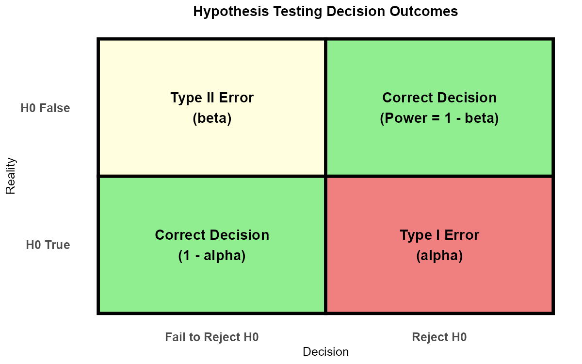
Fig. 10.31 The four possible outcomes in hypothesis testing: correct decisions vs. errors.

Part (a): What’s wrong

We never “accept” the null hypothesis. A large p-value means the data are consistent with H₀, but it doesn’t prove H₀ is true. Absence of evidence is not evidence of absence.

Part (b): Why “fail to reject”

• H₀ is assumed true from the start—we can’t “accept” what we already assumed

• A large p-value could result from H₀ being true OR from insufficient power to detect a false H₀

• The burden of proof is on rejecting H₀, not confirming it

• “Accept” implies certainty that isn’t justified

Part (c): Three reasons for failing to reject a false H₀

1. Sample size too small: Insufficient power to detect the true effect

2. Effect size too small: The true difference exists but is subtle

3. High variability: Large σ obscures the signal

4. Bad luck: Random sampling variation produced an unrepresentative sample (Type II error)

Part (d): Corrected conclusion

“The data does not give support (p-value = 0.45) to the claim that the mean differs from 100. The data are consistent with a mean of 100, but we cannot rule out other values.”

---

Exercise 5: Effect of Sample Size on Significance

Consider testing H₀: μ = 100 vs Hₐ: μ ≠ 100 with \(\bar{x} = 102\) and σ = 10.

1. Calculate the p-value for n = 25, 50, 100, 200, 400.

2. At what sample size does the result first become significant at α = 0.05?

3. The true difference (102 - 100 = 2) is the same in all cases. What does this tell you about the relationship between statistical significance and practical significance?

4. A researcher with n = 400 reports “highly significant results (p < 0.001).” What caution should readers exercise?

Solution

Part (a): P-values at different sample sizes

For each n: \(z_{TS} = \frac{102 - 100}{10/\sqrt{n}} = \frac{2\sqrt{n}}{10} = 0.2\sqrt{n}\)

n	z_TS	p-value (two-tailed)
25	1.00	0.3173
50	1.41	0.1573
100	2.00	0.0455
200	2.83	0.0047
400	4.00	0.00006

Part (b): First significant at α = 0.05

The result first becomes significant at n = 100 (p = 0.0455 < 0.05).

Part (c): Statistical vs practical significance

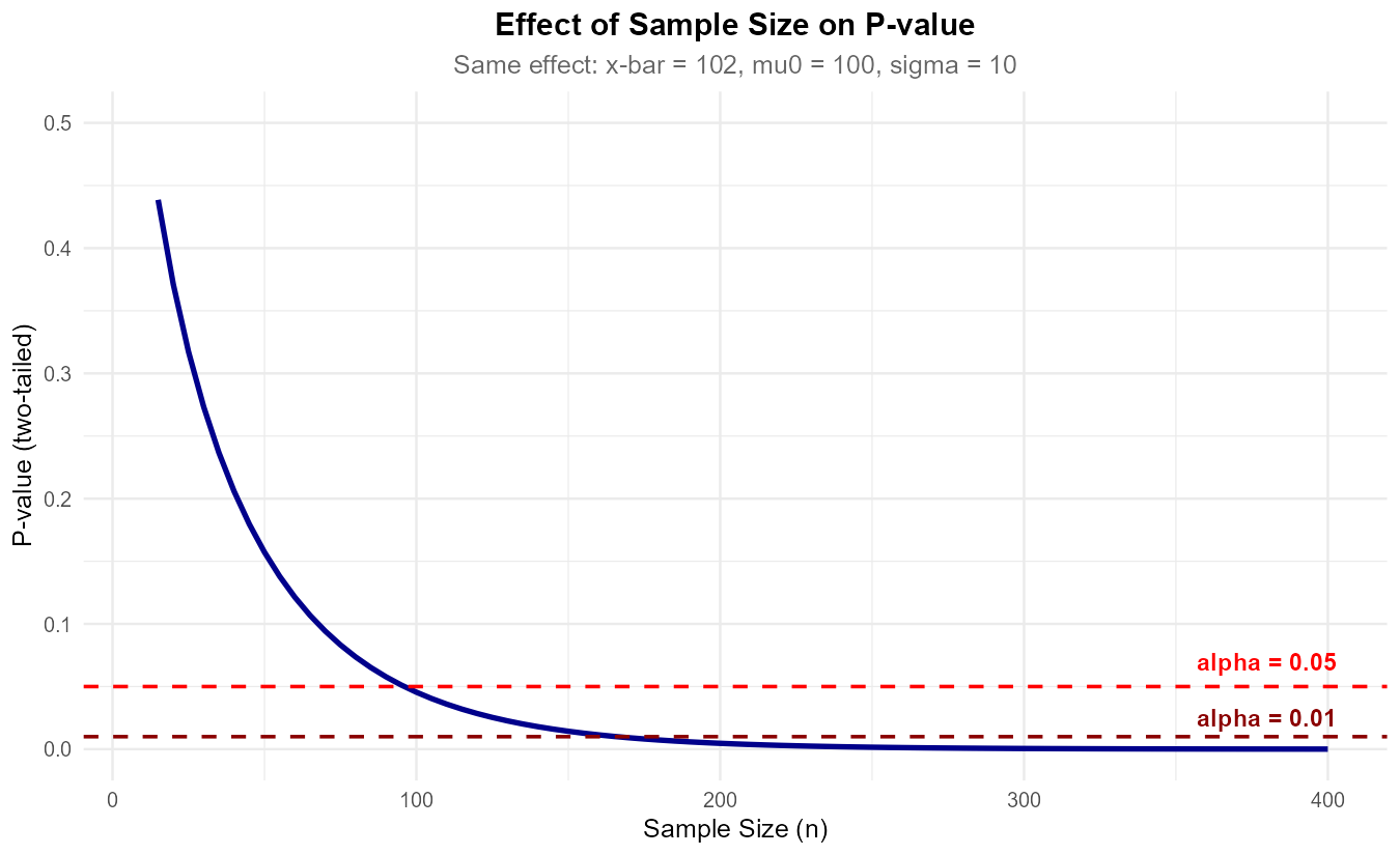
Fig. 10.32 With the same effect size, p-value decreases as sample size increases.

The effect size (2 points) is constant, but statistical significance depends heavily on sample size. With a large enough sample, even tiny, practically meaningless differences become statistically significant.

Key insight: Statistical significance ≠ practical importance. Always consider:

• Effect size (how big is the difference?)

• Confidence interval (what’s the range of plausible values?)

• Context (does this difference matter in practice?)

Part (d): Caution with large n

With n = 400, even a small effect (2 points out of 100) produces a highly significant p-value. Readers should:

• Ask about the effect size and whether it’s meaningful

• Look at the confidence interval (which would be narrow: approximately 101 to 103)

• Consider whether a 2% increase is practically important

• Not confuse “highly significant” with “large effect”

Best practice: Always report the estimated effect and a confidence interval, not just the p-value. A complete report would state: “The mean was 102 (95% CI: 101.0 to 103.0), representing a 2-point increase (p < 0.001).”

R verification:

xbar <- 102; mu_0 <- 100; sigma <- 10
n_values <- c(25, 50, 100, 200, 400)

for (n in n_values) {
  z_ts <- (xbar - mu_0) / (sigma / sqrt(n))
  p_val <- 2 * pnorm(abs(z_ts), lower.tail = FALSE)
  cat("n =", n, ": z =", round(z_ts, 2), ", p =", round(p_val, 4), "\n")
}

---

Exercise 6: Identifying P-value Hacking

For each scenario, identify whether p-value hacking (or questionable research practices) may be occurring. Explain why.

1. A researcher tests 20 different outcome variables and reports only the one with p < 0.05.

2. A researcher collects data until p < 0.05, then stops.

3. A researcher removes “outliers” that make the p-value larger.

4. A researcher pre-registers their hypothesis, sample size, and analysis plan before collecting data.

5. A researcher switches from a two-tailed to a one-tailed test after seeing the data.

6. A researcher reports “marginally significant results (p = 0.08)” as evidence supporting their hypothesis.

Solution

Part (a): Testing 20 outcomes, reporting 1 → P-VALUE HACKING

With 20 independent tests at α = 0.05, we expect about 1 false positive even if all null hypotheses are true. Selective reporting inflates the false positive rate. This should use multiple comparison corrections.

Part (b): Collecting until p < 0.05 → P-VALUE HACKING

“Optional stopping” inflates Type I error. The longer you keep sampling, the more likely you’ll eventually get p < 0.05 by chance. Sample size should be determined before data collection.

Part (c): Removing “outliers” to improve p → P-VALUE HACKING

If outlier removal is based on its effect on p-value (rather than pre-specified criteria like data entry errors), this is manipulation. Legitimate outlier handling should be decided before seeing results.

Part (d): Pre-registration → GOOD PRACTICE ✓

Pre-registering hypotheses and analysis plans prevents many forms of p-hacking. It makes the research transparent and ensures the analysis wasn’t tailored to get desired results.

Part (e): Switching to one-tailed after seeing data → P-VALUE HACKING

The test type should be determined by the research question before seeing data. Switching to one-tailed after observing the direction essentially halves the p-value, inflating false positives.

Part (f): “Marginally significant” p = 0.08 → QUESTIONABLE

While not strictly p-hacking, this represents “spin”—framing non-significant results as if they’re meaningful. The result did not meet the stated threshold. It’s honest to say “we found no significant effect (p = 0.08)” rather than implying near-success.

---

Exercise 7: Complete Four-Step Analysis

A coffee shop claims their large cups contain at least 16 oz of coffee. A consumer group suspects the cups are underfilled. They purchase n = 25 large coffees and measure:

• \(\bar{x} = 15.6\) oz

• s = 1.2 oz

Conduct a complete hypothesis test at α = 0.05 using the four-step framework.

Solution

Step 1: Define the Parameter

Let μ = true mean volume of coffee (oz) in large cups at this coffee shop.

Step 2: State the Hypotheses

The consumer group suspects underfilling (less than claimed):

\[H_0: \mu \geq 16 \quad \text{vs} \quad H_a: \mu < 16\]

This is a lower-tailed test.

Step 3: Calculate Test Statistic and P-value

Since σ is unknown, use t-test. df = 25 - 1 = 24.

\[t_{TS} = \frac{15.6 - 16}{1.2 / \sqrt{25}} = \frac{-0.4}{0.24} = -1.667\]

P-value (lower-tailed):

\[p\text{-value} = P(T_{24} < -1.667) = 0.0543\]

Step 4: Decision and Conclusion

Since p-value = 0.0543 > α = 0.05, fail to reject H₀.

Conclusion: The data does not give support (p-value = 0.054) to the claim that the mean coffee volume is less than 16 oz. While the sample mean (15.6 oz) is below the claimed amount, the difference is not statistically significant. The consumer group cannot definitively conclude underfilling based on this sample.

Note: The p-value is very close to 0.05. A slightly larger sample might yield significant results. The 95% UCB would be useful here.

R verification:

xbar <- 15.6; mu_0 <- 16; s <- 1.2; n <- 25
t_ts <- (xbar - mu_0) / (s / sqrt(n))  # -1.667
df <- n - 1  # 24
p_value <- pt(t_ts, df, lower.tail = TRUE)  # 0.0543

---

Exercise 8: Interpreting Non-significant Results

A clinical trial tests whether a new drug lowers blood pressure more than a placebo. With n = 30 patients per group, they find p = 0.15.

1. State the formal conclusion at α = 0.05.

2. A journalist writes: “Study proves new drug doesn’t work.” Is this accurate? Why or why not?

3. What are possible explanations for the non-significant result?

4. What would you recommend for follow-up research?

Solution

Part (a): Formal conclusion

At the 5% significance level, fail to reject H₀. The data does not give support (p-value = 0.15) to the claim that the new drug lowers blood pressure more than the placebo.

Part (b): Journalist’s interpretation

Not accurate. “Proves doesn’t work” overstates what we can conclude. Non-significance means:

• We failed to detect an effect, NOT that no effect exists

• The study may have been underpowered

• There could be a real but small effect

Better headline: “Study fails to find evidence that new drug works” or “Results inconclusive for new blood pressure drug.”

Part (c): Possible explanations

1. Drug truly doesn’t work (H₀ is true)

2. Underpowered study: n = 30 per group may be too small to detect a real effect

3. Effect size smaller than expected: The drug works but the effect is subtle

4. High variability: Individual differences in blood pressure response may obscure the drug effect

5. Wrong outcome measure: Perhaps the drug works but takes longer than the study period

6. Type II error: Random chance produced an unrepresentative sample

Part (d): Recommendations for follow-up

• Power analysis: Determine sample size needed to detect a clinically meaningful effect

• Larger study: Conduct a trial with adequate power (perhaps n = 100+ per group)

• Report effect size and CI: Even if non-significant, show the estimated effect and uncertainty

• Meta-analysis: Combine with other studies if available

• Explore subgroups: Some patient populations may respond differently

---

Exercise 9: Comprehensive Application

A university wants to evaluate whether a new tutoring program improves student performance. They randomly assign 40 students to receive tutoring and compare their exam scores to the historical mean of μ₀ = 72.

Results:

• n = 40

• \(\bar{x} = 75.8\)

• s = 12.5

1. Perform a complete hypothesis test at α = 0.05.

2. Calculate and interpret a 95% confidence interval.

3. A skeptic says: “A 3.8-point increase is trivial. This result is not practically significant.” How would you respond?

4. Another researcher notes: “But the p-value is barely below 0.05. This is weak evidence.” Evaluate this criticism.

5. What additional information would help evaluate the tutoring program’s effectiveness?

Solution

Part (a): Hypothesis Test

Step 1: Let μ = true mean exam score for students receiving tutoring.

Step 2: H₀: μ ≤ 72 vs Hₐ: μ > 72 (upper-tailed test)

Step 3:

\[t_{TS} = \frac{75.8 - 72}{12.5 / \sqrt{40}} = \frac{3.8}{1.976} = 1.923\]

df = 39

P-value = P(T₃₉ > 1.923) = 0.031

Step 4: Since 0.031 < 0.05, reject H₀.

At the 5% significance level, reject H₀. The data does give support (p-value = 0.031) to the claim that students receiving tutoring have a higher mean exam score than the historical average of 72.

Part (b): 95% Confidence Interval

t₀.₀₂₅,₃₉ = 2.023

\[CI: 75.8 \pm 2.023 \times 1.976 = 75.8 \pm 4.0 = (71.8, 79.8)\]

Interpretation: We are 95% confident that the true mean exam score for tutored students is between 71.8 and 79.8 points.

Part (c): Practical significance response

The skeptic raises a valid point. Statistical significance ≠ practical importance. To evaluate:

• Context matters: Is 3.8 points educationally meaningful? On a 100-point exam, it’s nearly 4%—potentially the difference between letter grades.

• Cost-benefit: How much does the tutoring cost? If inexpensive, even a modest improvement may be worthwhile.

• Effect size: Cohen’s d ≈ 3.8/12.5 = 0.30, a “small-to-medium” effect by conventional standards.

• The CI (71.8, 79.8) suggests the true effect could range from essentially zero to nearly 8 points.

Part (d): “Barely significant” criticism

This is a fair observation:

• P = 0.031 is not far from 0.05; with slightly different data, we might not reject

• The evidence, while meeting the threshold, is not overwhelming

• This underscores why we shouldn’t treat α = 0.05 as a magic cutoff

• Replication would strengthen confidence in the finding

Part (e): Additional information needed

• Control group: Were non-tutored students tested simultaneously? (Historical comparison is weaker than randomized control)

• Random assignment verification: How were students assigned to tutoring?

• Baseline scores: Were groups comparable before tutoring?

• Long-term effects: Do improvements persist?

• Cost analysis: What’s the cost per point of improvement?

• Subgroup analysis: Do some students benefit more than others?

• Multiple outcomes: What about other measures (retention, satisfaction)?

R verification:

xbar <- 75.8; mu_0 <- 72; s <- 12.5; n <- 40
SE <- s / sqrt(n)  # 1.976
t_ts <- (xbar - mu_0) / SE  # 1.923
df <- n - 1  # 39

# P-value
pt(t_ts, df, lower.tail = FALSE)  # 0.031

# 95% CI
t_crit <- qt(0.025, df, lower.tail = FALSE)  # 2.023
c(xbar - t_crit * SE, xbar + t_crit * SE)  # (71.8, 79.8)

---

10.4.7. Additional Practice Problems

True/False Questions (1 point each)

1. A p-value of 0.001 proves that H₀ is false.

   Ⓣ or Ⓕ

2. A large p-value (e.g., 0.60) means we should accept H₀.

   Ⓣ or Ⓕ

3. Statistical significance always implies practical significance.

   Ⓣ or Ⓕ

4. P-value hacking inflates the Type I error rate.

   Ⓣ or Ⓕ

5. With a large enough sample, virtually any small effect can become statistically significant.

   Ⓣ or Ⓕ

6. Pre-registration of studies helps prevent p-value hacking.

   Ⓣ or Ⓕ

Multiple Choice Questions (2 points each)

7. A p-value is defined as:

   Ⓐ The probability that H₀ is true

   Ⓑ The probability of the observed data, assuming H₀ is true

   Ⓒ The probability of data at least as extreme as observed, assuming H₀ is true

   Ⓓ The probability of making a Type I error

8. “Failing to reject H₀” means:

   Ⓐ H₀ is proven true

   Ⓑ Hₐ is proven false

   Ⓒ There is insufficient evidence to conclude Hₐ

   Ⓓ The test was conducted incorrectly

9. Which is an example of p-value hacking?

   Ⓐ Pre-registering hypotheses before data collection

   Ⓑ Using Bonferroni correction for multiple tests

   Ⓒ Removing outliers that make p larger

   Ⓓ Reporting non-significant results

10. A researcher finds p = 0.04 with n = 10,000. Which is the best interpretation?

    Ⓐ The effect is definitely large and important

    Ⓑ The result is statistically significant; effect size should be examined

    Ⓒ The null hypothesis is proven false

    Ⓓ The test was too conservative

11. A proper conclusion when p = 0.08 and α = 0.05 is:

    Ⓐ “We accept H₀”

    Ⓑ “The results are marginally significant”

    Ⓒ “There is insufficient evidence to reject H₀”

    Ⓓ “The alternative hypothesis is false”

12. Statistical significance depends on all EXCEPT:

    Ⓐ Sample size

    Ⓑ Effect size

    Ⓒ Population size

    Ⓓ Variability in the data

Answers to Practice Problems

True/False Answers:

1. False — No p-value can “prove” anything. Small p-values provide evidence against H₀ but could be Type I errors.

2. False — We never “accept” H₀. Large p-values mean insufficient evidence to reject.

3. False — A small p-value can arise from large n even when the effect is trivially small.

4. True — By selectively reporting or manipulating to get p < α, the actual false positive rate exceeds α.

5. True — SE = σ/√n decreases with n, so even tiny effects become significant with large n.

6. True — Pre-registration commits researchers to their analysis plan before seeing data.

Multiple Choice Answers:

7. Ⓒ — P-value = P(data at least as extreme as observed | H₀ true).

8. Ⓒ — Failing to reject means the evidence was insufficient, not that H₀ is true.

9. Ⓒ — Removing outliers based on their effect on p-value is manipulation.

10. Ⓑ — With n = 10,000, statistical significance is easy to achieve; effect size matters more.

11. Ⓒ — This is the proper phrasing when p > α.

12. Ⓒ — Population size doesn’t affect significance (except in finite population corrections rarely used). Sample size, effect size, and variability all matter.