Slides 📊

Download Chapter 7 slides (PPTX)

7.3. The Central Limit Theorem (CLT)

We’ve established that the sampling distribution of \(\bar{X}\) is normal when the population is normal. Then what about cases where the population is not normally distributed? The Central Limit Theorem (CLT) is a pivotal concept in statistics that addresses this question.

Road Map 🧭

• Learn the formal statement of the Central Limit Theorem (CLT).

• Recognize the experimental settings where the CLT applies.

• Apply the CLT to compute approximate probabilities of the sample mean.

7.3.1. The Formal Statement of the CLT

For an independent and identically distributed (iid) random sample \(X_1, X_2, ..., X_n\) from a population with a finite mean \(μ\) and finite standard deviation \(σ\),

\[\frac{\bar{X} - \mu}{\sigma/\sqrt{n}} \xrightarrow{d} N(0,1) \text{ as } n \rightarrow \infty\]

What does this all mean? 🔎

• \(\frac{\bar{X} - \mu}{\sigma/\sqrt{n}}\) is the standardized sample mean. \(\bar{X}\) is subtracted by its own mean \(\mu_{\bar{X}} = \mu\), then divided by its own standard deviation \(\sigma_{\bar{X}} = \frac{\sigma}{\sqrt{n}}\) (the standard error).

• \(\xrightarrow{d}\) indicates convergence in distribution.

• Putting together, the mathematical statement reads: “The distribution of the standardized sample mean approaches standard normal as the sample size \(n\) goes to infinity.”

Practical Implications of the CLT

When

1. the population has a finite mean \(\mu\) and a finite standard deviation \(\sigma\),

2. the observations are independent and identically distributed (iid), and

3. the sample size \(n\) is sufficiently large,

we have

\[\frac{\bar{X} - \mu}{\sigma/\sqrt{n}} \stackrel{d}{\approx} Z,\]

where \(\stackrel{d}{\approx}\) indicates that the two random variables have similar distributions. By applying the same linear operations on both sides, we can equivalently write:

\[\bar{X} \stackrel{d}{\approx} \frac{\sigma}{\sqrt{n}} Z + \mu.\]

The right-hand side is a linear transformation of a standard normal random variable with the distribution \(N(\mu, \sigma/\sqrt{n})\). It follows that:

\[\bar{X} \stackrel{\text{approx}}{\sim} N\left(\mu, \frac{\sigma}{\sqrt{n}}\right).\]

7.3.2. Visual Demonstrations

The Central Limit Theorem (CLT) states that the sampling distribution of the sample mean approaches a normal distribution as the sample size increases, regardless of the shape of the population distribution, as long as certain conditions are met. Let us use a visual tool to build intuition for this somewhat surprising result.

How to Use the Simulation Tool

The simulation tool requires a few inputs.

Argument	Description	How to use
Population Distribution	Normal, uniform, exponential, etc.	Select the family of distributions from which samples will be generated
Population Parameters	Different for each population family (e.g., \(\mu\) and \(\sigma\) for normal, \(\lambda\) for exponential)	Select the specific distribution belonging to the chosen family
Sample Size \(n\)	The number of data points used to compute one sample mean	Increase from small to large. Observe the change in the sampling distribution
Number of Samples	The number of different sample means used to construct a histogram of the sampling distribution	Fix at a large number (10000, for example) so the sampling distribution of of sample means is sufficiently described.

Once all values are set as desired, click simulate. Two plots will display:

• A pdf/pmf plot of the population distribution

• A histogram of sample means drawn from the population

Interactive Visualization 🎮

Central Limit Theorem Simulation

Visualize how sample means converge to a normal distribution as sample size increases, regardless of the underlying population distribution.

🔗 Launch Interactive Demo | 📄 View R Code

A Checklist

By experimenting with different settings, confirm the following:

✔❓	To confirm
	The CLT indeed holds. That is, the histogram of sample means approaches a normal shape as \(n\) grows.
	A large enough \(n\), which makes the histogram look sufficiently normal, is different for each population distribution. In general, a population requires a larger \(n\) if it has strong non-normal characteristics (asymetry, multimodality, etc.).
	the center of the histogram remains around \(\mu\) while the spread (\(\sigma/\sqrt{n}\)) narrows around \(\mu\) as \(n\) increases.

How Large is “Sufficiently Large”?

The common rule of thumb that n > 30 is sufficient should not be blindly applied. As we saw through simulations, the appropriate sample size depends entirely on the underlying population distribution. The farther the population distribution is from normal, the larger the sample size needed for the CLT to apply effectively.

In practice, we only observe a single sample from a population. Our understanding of the population depends on the sample we observe and our background knowledge. We must explore our sample carefully to determine if the sample size is likely sufficient for the CLT to apply.

7.3.3. Step-by-Step Problem Solving with the CLT

Problems using the CLT follow the general steps below:

1. Verify that the prerequisites for the CLT are met.

2. Identify the population mean \(\mu_X\) and standard deviation \(\sigma_X\), and use them to calculate the mean \(\mu_{\bar{X}} = \mu_X\) and the standard error \(\sigma_{\bar{X}} = \sigma_X/\sqrt{n}\) of the sampling distribution.

3. Establish the approximate sampling distribution of the sample mean: \(\bar{X} \stackrel{\text{approx}}{\sim} N(\mu_{\bar{X}}, \sigma_{\bar{X}})\).

4. Use a standard normal table or software to find the required probability.

Example💡: Another Maze Navigation Example

The same subspecies of rat from the previous experiment will be forced to navigate a more complex maze in which a wrong turn early on can drastically increase the time to completion. The true mean completion time for the whole population of the subspecies is known to be 10 minutes. The true standard deviation is 3 minutes. It is also known that the distribution is slightly right skewed.

Suppose that 60 rats are randomly selected from the population to navigate the maze.

1. What is the mean of the average time it takes 60 rats to navigate the maze?

2. What is the standard deviation of the average time?

3. What is the probability that the average maze navigation time for the 60 rats is greater than 11 minutes?

Organize the Given Information

We know that the distribution of the population \(X\) is slightly right skewed. Further, \(\mu_X=10\) and \(\sigma_X=3\).

Solve the Problems

1. \(\mu_{\bar{X}} = \mu_{X} = 10\)

2. \(\sigma_{\bar{X}} = \frac{\sigma_X}{\sqrt{n}} = \frac{3}{\sqrt{60}}=0.3878\)

3. We do not know the population distribution, so we hope to use the CLT to compute the probability. We must first confirm that all the conditions are met for the CLT to hold:

   1. The population mean and standard deviation are finite. ✔

   2. The sample was formed by taking random samples from the same population. The randmonness ensures that the selection of one rat does not influence others (independence). Since they come from the same population, their distributions are identical. ✔

   3. For a slightly skewed distribution, \(n=60\) is large enough. (To confirm, try plotting a left-skewed beta case with \(\alpha=3, \beta=2\) using the simulation tool above). ✔

   Therefore, \(\bar{X} \stackrel{\text{approx}}{\sim} N(\mu_{X}=10, \sigma_{\bar{X}}=0.3878)\) by the CLT. Then

   \[\begin{split}P(\bar{X} > 11) &= 1 - P(\bar{X} \leq 11) \\ &= 1 - P\left(Z \leq \frac{11-10}{3/\sqrt{60}}\right) \\ &= 1-\Phi(2.58) = 0.0049\end{split}\]

7.3.4. Bringing It All Together

Key Takeaways 📝

1. The Central Limit Theorem states that for an iid sample from a population with finite mean and variance, the distribution of the standardized sample mean approaches standard normal as the sample size increases.

2. The CLT can be used to approximate the sampling distribution of \(\bar{X}\), but the sample size needed depends on how far the population distribution deviates from normality.

The Central Limit Theorem represents one of the most powerful and remarkable results in statistics. It allows us to use the normal distribution as a foundation for statistical inference across a wide range of real-world situations, even when the underlying population distributions are unknown or non-normal.

7.3.5. Exercises

These exercises develop your skills in applying the Central Limit Theorem to approximate the sampling distribution of the sample mean when the population is not normally distributed.

Key Concepts

Central Limit Theorem (CLT): For an iid random sample from a population with finite mean \(\mu\) and finite standard deviation \(\sigma\), as \(n \to \infty\):

\[\frac{\bar{X} - \mu}{\sigma/\sqrt{n}} \xrightarrow{d} N(0,1)\]

Practical implication: When \(n\) is sufficiently large,

\[\bar{X} \stackrel{\text{approx}}{\sim} N\left(\mu, \sigma_{\bar{X}}^2\right) \quad \text{where } \sigma_{\bar{X}} = \frac{\sigma}{\sqrt{n}}\]

Throughout these exercises, \(N(\mu, \sigma^2)\) denotes a normal distribution with mean \(\mu\) and variance \(\sigma^2\).

CLT Conditions Checklist

Before applying the CLT, verify:

1. ✓ Population has finite mean \(\mu\) and finite standard deviation \(\sigma\)

2. ✓ Observations are independent and identically distributed (iid)

3. ✓ Sample size \(n\) is sufficiently large (depends on population shape)

Important: The required sample size depends heavily on how far the population deviates from normality. Symmetric populations may need only \(n \geq 15\), while heavily skewed or heavy-tailed distributions may require \(n \geq 50\) or more. The common “\(n \geq 30\)” rule is a rough guideline, not a guarantee.

R Functions for CLT Calculations

Once the CLT applies, use normal distribution functions with \(\mu_{\bar{X}} = \mu\) and \(\sigma_{\bar{X}} = \sigma/\sqrt{n}\):

# Define parameters
mu <- ...           # Population mean
sigma <- ...        # Population SD
n <- ...            # Sample size
se <- sigma / sqrt(n)  # Standard error

# Probability calculations for X̄
pnorm(x, mean = mu, sd = se)                     # P(X̄ ≤ x)
pnorm(x, mean = mu, sd = se, lower.tail = FALSE) # P(X̄ > x)

# Quantiles of X̄
qnorm(p, mean = mu, sd = se)                     # Find x such that P(X̄ ≤ x) = p

Exercise 1: CLT with Uniform Population

The time (in seconds) for a random number generator to complete a cryptographic operation follows a uniform distribution on the interval \([2, 6]\).

1. Find the population mean \(\mu\) and population standard deviation \(\sigma\).

2. For a sample of \(n = 49\) operations, find the mean and standard error of \(\bar{X}\).

3. Verify that the CLT conditions are satisfied.

4. Use the CLT to approximate \(P(\bar{X} > 4.2)\).

5. Find \(P(3.7 < \bar{X} < 4.3)\).

Solution

Let \(X\) = time for one operation (seconds), where \(X \sim \text{Uniform}(2, 6)\).

Part (a): Population parameters

For a uniform distribution on \([a, b]\):

\[\mu = \frac{a + b}{2} = \frac{2 + 6}{2} = 4 \text{ seconds}\]

\[\sigma = \frac{b - a}{\sqrt{12}} = \frac{6 - 2}{\sqrt{12}} = \frac{4}{3.464} = 1.155 \text{ seconds}\]

Part (b): Sampling distribution parameters

\[\mu_{\bar{X}} = \mu = 4 \text{ seconds}\]

\[\sigma_{\bar{X}} = \frac{\sigma}{\sqrt{n}} = \frac{1.155}{\sqrt{49}} = \frac{1.155}{7} = 0.165 \text{ seconds}\]

Part (c): CLT conditions

1. ✓ Finite mean and SD: \(\mu = 4\) and \(\sigma = 1.155\) are both finite.

2. ✓ iid: Operations are randomly selected and independent of each other under stable conditions.

3. ✓ Sample size: The uniform distribution is symmetric and bounded, so the CLT converges quickly. With \(n = 49\), the normal approximation is excellent.

Part (d): P(X̄ > 4.2) using CLT

By CLT: \(\bar{X} \stackrel{\text{approx}}{\sim} N(4, 0.165^2)\).

\[P(\bar{X} > 4.2) = P\left(Z > \frac{4.2 - 4}{0.165}\right) = P(Z > 1.21)\]

\[= 1 - \Phi(1.21) = 1 - 0.8869 = 0.1131\]

Part (e): P(3.7 < X̄ < 4.3)

\[P(3.7 < \bar{X} < 4.3) = P\left(\frac{3.7 - 4}{0.165} < Z < \frac{4.3 - 4}{0.165}\right)\]

\[= P(-1.82 < Z < 1.82) = \Phi(1.82) - \Phi(-1.82)\]

\[= 0.9656 - 0.0344 = 0.9312\]

R verification:

mu <- 4
sigma <- 4/sqrt(12)  # 1.1547
n <- 49
se <- sigma / sqrt(n)  # 0.1650

# Part (d): P(X̄ > 4.2)
pnorm(4.2, mean = mu, sd = se, lower.tail = FALSE)
# [1] 0.1127

# Part (e): P(3.7 < X̄ < 4.3)
pnorm(4.3, mean = mu, sd = se) - pnorm(3.7, mean = mu, sd = se)
# [1] 0.9310

---

Exercise 2: CLT with Exponential Population

The time between customer arrivals at a help desk follows an exponential distribution with mean \(\mu = 5\) minutes.

1. What is the population standard deviation \(\sigma\)?

2. A manager records \(n = 40\) inter-arrival times and computes the sample mean. What is the approximate distribution of \(\bar{X}\)?

3. Find the probability that the sample mean inter-arrival time is less than 4 minutes.

4. Find the probability that the sample mean is within 1 minute of the population mean.

5. The exponential distribution is right-skewed. Why is \(n = 40\) likely sufficient for the CLT approximation?

Solution

Let \(X\) = inter-arrival time (minutes), where \(X \sim \text{Exp}(\mu = 5)\).

Part (a): Population standard deviation

For an exponential distribution, \(\sigma = \mu\) (a unique property of this distribution).

\[\sigma = 5 \text{ minutes}\]

Part (b): Approximate distribution of X̄

First, calculate the standard error:

\[\sigma_{\bar{X}} = \frac{\sigma}{\sqrt{n}} = \frac{5}{\sqrt{40}} = \frac{5}{6.325} = 0.791 \text{ minutes}\]

CLT conditions check:

1. ✓ Finite mean (\(\mu = 5\)) and SD (\(\sigma = 5\))

2. ✓ iid: Inter-arrival times are independent and from the same process

3. ✓ \(n = 40\) is reasonably large for moderately skewed exponential

By CLT:

\[\bar{X} \stackrel{\text{approx}}{\sim} N(5, 0.791^2)\]

Part (c): P(X̄ < 4)

\[P(\bar{X} < 4) = P\left(Z < \frac{4 - 5}{0.791}\right) = P(Z < -1.26)\]

\[= \Phi(-1.26) = 0.1038\]

Part (d): P(|X̄ − μ| < 1) = P(4 < X̄ < 6)

\[P(4 < \bar{X} < 6) = P\left(\frac{4 - 5}{0.791} < Z < \frac{6 - 5}{0.791}\right)\]

\[= P(-1.26 < Z < 1.26) = \Phi(1.26) - \Phi(-1.26)\]

\[= 0.8962 - 0.1038 = 0.7924\]

R verification:

mu <- 5
sigma <- 5  # For exponential, σ = μ
n <- 40
se <- sigma / sqrt(n)  # 0.7906

# Part (c): P(X̄ < 4)
pnorm(4, mean = mu, sd = se)
# [1] 0.1034

# Part (d): P(4 < X̄ < 6)
pnorm(6, mean = mu, sd = se) - pnorm(4, mean = mu, sd = se)
# [1] 0.7932

Part (e): Why n = 40 is likely sufficient

Although the exponential distribution is right-skewed, it has moderate skewness (skewness coefficient = 2 for all exponential distributions). The CLT converges reasonably quickly for such distributions. With \(n = 40\), the averaging process is often adequate for many practical probability calculations involving the exponential distribution. However, for populations with more extreme skewness or heavier tails, larger samples may be needed.

---

Exercise 3: Effect of Sample Size on CLT Approximation

A manufacturing process produces components with weights that follow a right-skewed distribution with \(\mu = 50\) grams and \(\sigma = 8\) grams.

1. For \(n = 16\), find \(\sigma_{\bar{X}}\) and use the CLT to approximate \(P(\bar{X} > 52)\).

2. For \(n = 64\), find \(\sigma_{\bar{X}}\) and approximate \(P(\bar{X} > 52)\).

3. For \(n = 256\), find \(\sigma_{\bar{X}}\) and approximate \(P(\bar{X} > 52)\).

4. Explain the pattern in your answers. Why does \(P(\bar{X} > 52)\) decrease as \(n\) increases?

5. A quality engineer questions whether the CLT approximation is valid for \(n = 16\) given the skewed population. Is this concern reasonable?

Solution

Given: \(\mu = 50\) g, \(\sigma = 8\) g, population is right-skewed.

Part (a): n = 16

\[\sigma_{\bar{X}} = \frac{8}{\sqrt{16}} = 2 \text{ g}\]

By CLT: \(\bar{X} \stackrel{\text{approx}}{\sim} N(50, 2^2)\).

\[P(\bar{X} > 52) \approx P\left(Z > \frac{52 - 50}{2}\right) = P(Z > 1.00) = 1 - 0.8413 = 0.1587\]

Part (b): n = 64

\[\sigma_{\bar{X}} = \frac{8}{\sqrt{64}} = 1 \text{ g}\]

\[P(\bar{X} > 52) \approx P\left(Z > \frac{52 - 50}{1}\right) = P(Z > 2.00) = 1 - 0.9772 = 0.0228\]

Part (c): n = 256

\[\sigma_{\bar{X}} = \frac{8}{\sqrt{256}} = 0.5 \text{ g}\]

\[P(\bar{X} > 52) \approx P\left(Z > \frac{52 - 50}{0.5}\right) = P(Z > 4.00) \approx 0.00003\]

R verification:

mu <- 50
sigma <- 8

# Part (a): n = 16
pnorm(52, mean = mu, sd = sigma/sqrt(16), lower.tail = FALSE)
# [1] 0.1587

# Part (b): n = 64
pnorm(52, mean = mu, sd = sigma/sqrt(64), lower.tail = FALSE)
# [1] 0.02275

# Part (c): n = 256
pnorm(52, mean = mu, sd = sigma/sqrt(256), lower.tail = FALSE)
# [1] 3.167e-05

Part (d): Pattern explanation

\(n\)	\(\sigma_{\bar{X}}\)	\(P(\bar{X} > 52)\)
16	2.0 g	0.1587
64	1.0 g	0.0228
256	0.5 g	0.00003

As \(n\) increases, the standard error decreases, making the sampling distribution more concentrated around \(\mu = 50\). A value of 52 (which is 2 grams above the mean) becomes increasingly “extreme” in terms of standard errors: 1.0 SE for \(n = 16\), 2.0 SE for \(n = 64\), and 4.0 SE for \(n = 256\).

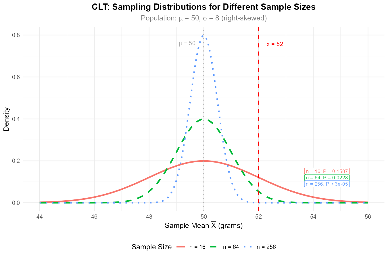
Fig. 7.6 Larger samples produce more concentrated sampling distributions, making P(X̄ > 52) decrease dramatically.

Part (e): Validity concern for n = 16

Yes, this concern is reasonable. For skewed populations, \(n = 16\) may not be large enough for the CLT approximation to be accurate. The approximation for \(n = 16\) should be treated as rough—directionally correct but potentially inaccurate depending on the degree of skewness and presence of outliers.

The results for \(n = 64\) and \(n = 256\) are more reliable. If high precision is needed with small samples from skewed populations, alternative methods (like bootstrapping) or larger sample sizes should be considered.

---

Exercise 4: Verifying CLT Conditions

For each scenario, determine whether the CLT can be appropriately applied. If not, explain which condition is violated.

1. Sample of 50 household incomes from a city, used to estimate mean income. Income distributions are typically right-skewed.

2. Sample of 25 measurements from a symmetric, bell-shaped population.

3. Sample of 100 observations from a manufacturing process, where each observation is the maximum of 10 temperature readings from the same set of correlated sensors taken in overlapping time windows.

4. Sample of 40 waiting times from a process that occasionally produces extreme outliers (heavy-tailed distribution with infinite variance).

5. Sample of 35 reaction times from a mildly skewed distribution with \(\mu = 250\) ms and \(\sigma = 40\) ms.

Solution

Part (a): Household incomes, n = 50, right-skewed

✓ CLT can be applied. Income distributions have finite mean and variance. With \(n = 50\), the sample size is large enough to handle right-skewness. The CLT approximation should be reasonably accurate.

Part (b): Bell-shaped population, n = 25

✓ CLT is valid, but not necessary. Since the population is symmetric and bell-shaped (approximately normal), the sampling distribution of \(\bar{X}\) is already approximately normal even for small \(n\). The exact normal result from Section 7.2 applies if the population is truly normal; otherwise, the CLT provides additional justification.

Part (c): Maximum of correlated sensors with overlapping windows, n = 100

✗ CLT cannot be applied. The observations are not independent—each observation is derived from the same set of correlated sensors, and overlapping time windows introduce temporal dependence between consecutive observations. The independence condition is violated. Even with \(n = 100\), the CLT does not apply because the variance formula \(\text{Var}(\bar{X}) = \sigma^2/n\) assumes independence; with dependent observations, the true variance of \(\bar{X}\) may be much larger.

Part (d): Heavy-tailed distribution with infinite variance, n = 40

✗ CLT cannot be applied. The CLT requires finite variance. If the population variance is infinite (as with some heavy-tailed distributions like the Cauchy distribution), the CLT does not hold regardless of sample size. The sampling distribution of \(\bar{X}\) will not approach normality.

Part (e): Mildly skewed reaction times, n = 35

✓ CLT can be applied. The population has finite \(\mu\) and \(\sigma\), observations can be assumed iid if properly sampled, and \(n = 35\) is reasonable for a mildly skewed distribution. With \(\sigma_{\bar{X}} = 40/\sqrt{35} = 6.76\) ms, the approximation \(\bar{X} \stackrel{\text{approx}}{\sim} N(250, 6.76^2)\) is reasonable.

---

Exercise 5: Comparing CLT to Normal Population Result

Consider two populations, both with \(\mu = 100\) and \(\sigma = 20\):

• Population A: Normally distributed

• Population B: Uniformly distributed on \([100 - 20\sqrt{3}, 100 + 20\sqrt{3}]\)

For samples of size \(n = 36\) from each population:

1. What is the sampling distribution of \(\bar{X}\) for Population A? (Use exact result.)

2. What is the approximate sampling distribution of \(\bar{X}\) for Population B? (Use CLT.)

3. Calculate \(P(\bar{X} < 95)\) for each population.

4. Why are the answers to part (c) similar?

Solution

Both populations have \(\mu = 100\), \(\sigma = 20\), and \(n = 36\).

Standard error: \(\sigma_{\bar{X}} = \frac{20}{\sqrt{36}} = \frac{20}{6} = 3.333\).

Part (a): Population A (Normal) — Exact result

Since Population A is normal, by the exact result from Section 7.2:

\[\bar{X} \sim N(100, 3.333^2) \quad \text{(exactly)}\]

Part (b): Population B (Uniform) — CLT approximation

The uniform distribution is symmetric with finite mean and variance, and \(n = 36\) is large. By CLT:

\[\bar{X} \stackrel{\text{approx}}{\sim} N(100, 3.333^2)\]

Part (c): P(X̄ < 95) for each population

Population A (exact):

\[P(\bar{X} < 95) = P\left(Z < \frac{95 - 100}{3.333}\right) = P(Z < -1.50) = 0.0668\]

Population B (CLT approximation):

\[P(\bar{X} < 95) \approx P\left(Z < \frac{95 - 100}{3.333}\right) = P(Z < -1.50) \approx 0.0668\]

R verification:

mu <- 100
se <- 20 / sqrt(36)  # 3.333

# Both populations give the same result
pnorm(95, mean = mu, sd = se)
# [1] 0.0668

Part (d): Why are the answers similar?

The answers are nearly identical because:

1. Both sampling distributions have the same mean (\(\mu_{\bar{X}} = 100\)) and standard error (\(\sigma_{\bar{X}} = 3.333\))

2. For Population A, normality is exact; for Population B, the CLT approximation is very accurate because the uniform distribution is symmetric and bounded, causing rapid convergence to normality

3. The CLT tells us that the shape of the population matters less and less as \(n\) increases—all sampling distributions converge to normal

This illustrates the power of the CLT: regardless of the original population shape, sample means behave similarly for large \(n\).

---

Exercise 6: Sample Size Determination

A quality control engineer needs to estimate the mean fill volume of bottles. The filling process has \(\sigma = 2.4\) mL, and the distribution is slightly right-skewed.

1. The engineer wants \(P(|\bar{X} - \mu| < 0.5) \geq 0.95\). Using the CLT approximation, find the minimum sample size needed.

2. Given that the population is skewed, should the engineer use a sample size larger than the minimum calculated in part (a)? Explain.

3. If the engineer uses \(n = 100\), find \(P(|\bar{X} - \mu| < 0.5)\).

Solution

Given: \(\sigma = 2.4\) mL, population slightly right-skewed.

Part (a): Minimum sample size for P(|X̄ − μ| < 0.5) ≥ 0.95

We need:

\[P\left(-0.5 < \bar{X} - \mu < 0.5\right) \geq 0.95\]

Standardizing:

\[P\left(-\frac{0.5}{\sigma_{\bar{X}}} < Z < \frac{0.5}{\sigma_{\bar{X}}}\right) \geq 0.95\]

For a symmetric interval, we need \(\frac{0.5}{\sigma_{\bar{X}}} \geq z_{0.975} = 1.96\).

\[\sigma_{\bar{X}} \leq \frac{0.5}{1.96} = 0.2551\]

\[\frac{2.4}{\sqrt{n}} \leq 0.2551 \implies \sqrt{n} \geq \frac{2.4}{0.2551} = 9.408 \implies n \geq 88.5\]

Minimum sample size: n = 89.

Part (b): Should a larger sample be used?

Yes, a larger sample is advisable for two reasons:

1. CLT accuracy: The calculation assumes the CLT approximation is accurate. For a skewed population, using a sample size larger than the theoretical minimum (e.g., \(n = 100\) or more) helps ensure the normal approximation is valid.

2. Safety margin: The minimum of 89 achieves exactly 95% probability under ideal conditions. Real-world variability and the approximation nature of the CLT suggest building in a buffer.

Part (c): P(|X̄ − μ| < 0.5) with n = 100

\[\sigma_{\bar{X}} = \frac{2.4}{\sqrt{100}} = 0.24 \text{ mL}\]

\[P(|\bar{X} - \mu| < 0.5) = P\left(-\frac{0.5}{0.24} < Z < \frac{0.5}{0.24}\right)\]

\[= P(-2.08 < Z < 2.08) = \Phi(2.08) - \Phi(-2.08)\]

\[= 0.9812 - 0.0188 = 0.9624\]

With \(n = 100\), there is about a 96.2% probability that the sample mean is within 0.5 mL of the true mean—exceeding the 95% target.

R verification:

sigma <- 2.4

# Part (a): Find minimum n for P(|X̄ - μ| < 0.5) ≥ 0.95
# Need SE ≤ 0.5/1.96
(2.4 / (0.5/qnorm(0.975)))^2
# [1] 88.5 → round up to 89

# Part (c): P(|X̄ - μ| < 0.5) with n = 100
se <- sigma / sqrt(100)  # 0.24
pnorm(0.5/se) - pnorm(-0.5/se)
# [1] 0.9625

---

Exercise 7: Process Monitoring Application

A chemical reactor operates with a temperature that fluctuates according to a distribution with \(\mu = 350°C\) and \(\sigma = 12°C\). The distribution is symmetric but has heavier tails than normal. Every hour, an automated system records \(n = 36\) temperature readings and computes the average.

1. Using the CLT, what is the approximate distribution of the hourly average temperature \(\bar{X}\)?

2. The system triggers an alert if \(\bar{X}\) falls outside the interval \([346, 354]\). What is the probability of a false alarm (alert when the process is operating normally)?

3. Suppose the reactor drifts so that \(\mu = 355°C\). What is the probability that the monitoring system detects this drift (i.e., \(\bar{X}\) falls outside \([346, 354]\))?

4. How would increasing \(n\) to 64 affect the false alarm rate and detection probability?

Solution

Given: \(\mu = 350°C\), \(\sigma = 12°C\), \(n = 36\), symmetric heavy-tailed distribution.

Part (a): Approximate distribution of X̄

Standard error: \(\sigma_{\bar{X}} = \frac{12}{\sqrt{36}} = 2°C\).

CLT conditions: ✓ Finite \(\mu\) and \(\sigma\), ✓ iid readings, ✓ \(n = 36\) is sufficient for a symmetric distribution (even with heavy tails, symmetry helps).

\[\bar{X} \stackrel{\text{approx}}{\sim} N(350, 2^2)\]

Part (b): False alarm probability when μ = 350

\[P(\text{false alarm}) = P(\bar{X} < 346 \text{ or } \bar{X} > 354)\]

\[= P\left(Z < \frac{346 - 350}{2}\right) + P\left(Z > \frac{354 - 350}{2}\right)\]

\[= P(Z < -2) + P(Z > 2) = 0.0228 + 0.0228 = 0.0456\]

About 4.56% false alarm rate.

Part (c): Detection probability when μ = 355

Now \(\bar{X} \stackrel{\text{approx}}{\sim} N(355, 2^2)\).

\[P(\text{detection}) = P(\bar{X} < 346 \text{ or } \bar{X} > 354)\]

\[= P\left(Z < \frac{346 - 355}{2}\right) + P\left(Z > \frac{354 - 355}{2}\right)\]

\[= P(Z < -4.5) + P(Z > -0.5)\]

\[\approx 0 + (1 - 0.3085) = 0.6915\]

About 69% detection rate—the system will catch the drift about 69% of the time.

Part (d): Effect of increasing n to 64

New standard error: \(\sigma_{\bar{X}} = \frac{12}{\sqrt{64}} = 1.5°C\).

False alarm rate (μ = 350):

\[P(Z < -2.67 \text{ or } Z > 2.67) = 2 \times 0.0038 = 0.0076 \approx 0.76\%\]

Detection rate (μ = 355):

\[P\left(Z < \frac{346-355}{1.5}\right) + P\left(Z > \frac{354-355}{1.5}\right) = P(Z < -6) + P(Z > -0.67)\]

\[\approx 0 + 0.7486 = 0.749 \approx 75\%\]

Summary: Increasing \(n\) from 36 to 64 decreases the false alarm rate (4.56% → 0.76%) while increasing the detection rate (69% → 75%). Larger samples make the monitoring system both more reliable and more sensitive.

R verification:

sigma <- 12

# With n = 36
se36 <- sigma / sqrt(36)  # 2
# Part (b): False alarm rate when μ = 350
pnorm(346, mean = 350, sd = se36) + pnorm(354, mean = 350, sd = se36, lower.tail = FALSE)
# [1] 0.0455

# Part (c): Detection rate when μ = 355
pnorm(346, mean = 355, sd = se36) + pnorm(354, mean = 355, sd = se36, lower.tail = FALSE)
# [1] 0.6915

# Part (d): With n = 64
se64 <- sigma / sqrt(64)  # 1.5
# False alarm rate
pnorm(346, mean = 350, sd = se64) + pnorm(354, mean = 350, sd = se64, lower.tail = FALSE)
# [1] 0.0076
# Detection rate
pnorm(346, mean = 355, sd = se64) + pnorm(354, mean = 355, sd = se64, lower.tail = FALSE)
# [1] 0.7475

---

Exercise 8: Exploring the CLT with Simulation 🎮

Use the interactive CLT simulation to explore how the sampling distribution of \(\bar{X}\) changes with different populations and sample sizes.

Access the simulation: CLT Interactive Demo

Setup: Set “Number of Samples (SRS)” to 10000 for all explorations (this ensures smooth histograms).

Part A: Effect of Sample Size on Convergence

1. Select Exponential distribution. Set \(n = 5\). Click Simulate.

   • Describe the shape of the sampling distribution histogram. Is it symmetric or skewed?

   • Compare the experimental mean and SD to the theoretical values.

2. Increase to \(n = 15\), then \(n = 30\), then \(n = 60\). For each:

   • How does the histogram shape change?

   • How does the QQ plot change? (Points closer to the line indicate better normality.)

3. At what sample size does the sampling distribution appear approximately normal for the exponential population?

Part B: Comparing Population Shapes

Using \(n = 30\) for each, compare the sampling distributions for:

1. Uniform — symmetric, bounded

2. Exponential — right-skewed, unbounded

3. Beta (try different α, β values) — can be skewed or symmetric

4. Bimodal — two peaks

For which population(s) does \(n = 30\) seem sufficient for normality? For which might you want a larger sample?

Part C: When CLT Fails

1. Select Cauchy (CLT Failure!) distribution with \(n = 30\). Simulate.

   • Does the sampling distribution look normal?

   • What happens to the experimental mean and SD across different simulations? (Click Simulate several times.)

2. Increase to \(n = 100\), then \(n = 500\). Does the sampling distribution become more normal?

3. Explain why the CLT fails for the Cauchy distribution.

Solution

Part A: Effect of Sample Size

1. n = 5 (Exponential): The histogram is noticeably right-skewed, similar to the population. The QQ plot shows curvature, indicating departure from normality. Experimental mean and SD should be close to theoretical values.

2. As n increases:

   • \(n = 15\): Still somewhat skewed but less pronounced

   • \(n = 30\): Approximately symmetric, QQ plot mostly linear

   • \(n = 60\): Very close to normal, QQ plot nearly perfect line

3. For the exponential distribution, \(n \approx 30\text{--}40\) typically produces an approximately normal sampling distribution. This aligns with the common rule of thumb.

Part B: Comparing Population Shapes

With \(n = 30\):

• Uniform: Sampling distribution is very close to normal. The uniform distribution is symmetric and bounded, so convergence is rapid. Even \(n = 10\text{--}15\) often suffices.

• Exponential: Approximately normal at \(n = 30\) for many practical calculations, though slight right skewness may still be visible in the QQ plot.

• Beta: Depends on parameters. Symmetric beta (\(\alpha = \beta\)) converges quickly; highly skewed beta (e.g., \(\alpha = 1, \beta = 5\)) may benefit from \(n > 30\text{--}40\).

• Bimodal: Often converges reasonably well by \(n = 30\) because averaging smooths out the two modes.

Key insight: The more the population deviates from normality (especially skewness and heavy tails), the larger the sample size needed for an accurate approximation.

Part C: When CLT Fails (Cauchy)

1. n = 30: The sampling distribution does NOT look normal. It has heavy tails and extreme outliers. The histogram may look erratic.

2. n = 100, 500: The distribution still does not become normal. You may see extreme sample means far from 0.

3. Experimental mean/SD instability: Each time you simulate, the experimental mean and SD change dramatically—they don’t stabilize.

Why CLT fails for Cauchy: The Cauchy distribution has no finite mean or variance (both are undefined/infinite). The CLT requires finite mean and variance. Without these, the sample mean does not converge to any distribution—it remains unstable and heavy-tailed regardless of sample size.

This demonstrates that the CLT conditions are not just technicalities—they are essential requirements.

---

Exercise 9: Conceptual Understanding

Answer the following conceptual questions about the Central Limit Theorem.

1. The CLT says the sampling distribution of \(\bar{X}\) approaches normal as \(n \to \infty\). Does this mean that individual observations \(X_i\) become more normal as we collect more data? Explain.

2. Two populations have the same mean and variance, but Population A is symmetric while Population B is heavily right-skewed. For which population would you need a larger sample size for the CLT approximation to be accurate? Why?

3. If a population is already normally distributed, is the CLT still useful? Explain.

4. A student claims: “The CLT guarantees that \(\bar{X}\) is normally distributed for any sample size as long as \(n \geq 30\).” Is this statement accurate? Critique it.

5. Based on the simulation in Exercise 8, explain why the Cauchy distribution is a counterexample to the CLT.

Solution

Part (a): Do individual observations become more normal?

No. The CLT describes the behavior of the sample mean \(\bar{X}\), not individual observations. The population distribution (and hence each \(X_i\)) remains unchanged regardless of sample size. The “magic” of the CLT is that averaging many observations produces a quantity that is approximately normal, even though the individual observations may be far from normal.

Part (b): Which population needs larger n?

Population B (heavily right-skewed) requires a larger sample size. The CLT converges faster for distributions that are closer to normal. Symmetric distributions converge quickly (often \(n \geq 15\text{--}20\) suffices), while heavily skewed distributions may need \(n \geq 50\) or more. The greater the departure from normality, the larger the \(n\) needed.

Part (c): Is the CLT useful for normal populations?

When the population is normal, we have the exact result from Section 7.2: \(\bar{X} \sim N(\mu, \sigma^2/n)\) for any sample size. The CLT is not needed in this case because we already know the exact distribution.

However, the CLT provides reassurance that our inference methods remain valid even if our normality assumption is slightly wrong—the procedures are robust to mild departures from normality.

Part (d): Critique of the “n ≥ 30” claim

This statement is not accurate. Issues include:

1. “Guarantees” is too strong—the CLT provides an approximation, not an exact result. The quality of the approximation depends on the population shape.

2. “n ≥ 30” is an oversimplified rule of thumb, not a universal threshold. Symmetric, bounded populations may need much less (even \(n = 10\text{--}15\)); heavily skewed or heavy-tailed populations may need \(n \geq 50\) or more.

3. The CLT describes what happens as \(n \to \infty\). For finite \(n\), we only have an approximation, and we should assess whether that approximation is adequate for our purposes.

A more accurate statement: “The required sample size for an adequate CLT approximation depends on the population’s departure from normality. Symmetric populations converge quickly; skewed or heavy-tailed populations require larger samples.”

Part (e): Cauchy as CLT counterexample

The Cauchy distribution has undefined (infinite) mean and variance. In Exercise 8’s simulation, we observed that:

• The sampling distribution of \(\bar{X}\) does not become more normal as \(n\) increases

• The experimental mean and SD are unstable across simulations

• Extreme outliers persist even with large samples

This occurs because the CLT requires finite mean and variance. The Cauchy distribution violates both conditions, so the theorem simply does not apply. This is not a matter of needing a “larger n”—the CLT will never work for Cauchy regardless of sample size.

---

7.3.6. Additional Practice Problems

True/False Questions (1 point each)

1. The Central Limit Theorem requires the population to be normally distributed.

   Ⓣ or Ⓕ

2. As sample size increases, the sampling distribution of \(\bar{X}\) becomes more concentrated around \(\mu\).

   Ⓣ or Ⓕ

3. The CLT can be applied when the population has infinite variance.

   Ⓣ or Ⓕ

4. For a symmetric population, a smaller sample size is typically needed for the CLT approximation to be accurate compared to a skewed population.

   Ⓣ or Ⓕ

5. The CLT tells us that individual observations become approximately normal when the sample size is large.

   Ⓣ or Ⓕ

6. If observations are not independent, the CLT does not apply.

   Ⓣ or Ⓕ

Multiple Choice Questions (2 points each)

7. The CLT states that as \(n \to \infty\), which quantity approaches a standard normal distribution?

   Ⓐ \(\bar{X}\)

   Ⓑ \(\frac{\bar{X} - \mu}{\sigma}\)

   Ⓒ \(\frac{\bar{X} - \mu}{\sigma/\sqrt{n}}\)

   Ⓓ \(\frac{X_i - \mu}{\sigma}\)

8. A population has \(\mu = 80\) and \(\sigma = 15\). For \(n = 25\), the CLT approximation gives \(\bar{X} \stackrel{\text{approx}}{\sim}\):

   Ⓐ \(N(80, 15^2)\)

   Ⓑ \(N(80, 3^2)\)

   Ⓒ \(N(80, 0.6^2)\)

   Ⓓ \(N(3.2, 80)\)

9. Which condition is NOT required for the CLT to apply?

   Ⓐ Population has finite mean

   Ⓑ Population has finite variance

   Ⓒ Population is normally distributed

   Ⓓ Observations are independent

10. For a heavily right-skewed population, which sample size is most likely to give an accurate CLT approximation?

    Ⓐ \(n = 10\)

    Ⓑ \(n = 25\)

    Ⓒ \(n = 50\)

    Ⓓ \(n = 100\)

11. If \(X \sim \text{Uniform}(0, 12)\), then \(\sigma =\):

    Ⓐ 6

    Ⓑ \(12/\sqrt{12} \approx 3.46\)

    Ⓒ 12

    Ⓓ 4

12. Using the CLT with \(\mu = 50\), \(\sigma = 10\), and \(n = 100\), find \(P(\bar{X} > 52)\):

    Ⓐ \(P(Z > 0.2)\)

    Ⓑ \(P(Z > 2)\)

    Ⓒ \(P(Z > 20)\)

    Ⓓ \(P(Z > 0.02)\)

Answers to Practice Problems

True/False Answers:

1. False — The CLT applies to any population with finite mean and variance, regardless of its distribution shape.

2. True — The standard error \(\sigma/\sqrt{n}\) decreases as \(n\) increases, concentrating the distribution around \(\mu\).

3. False — The CLT requires finite variance. For populations with infinite variance (like Cauchy), the CLT does not apply.

4. True — Symmetric distributions are “closer” to normal, so the CLT approximation converges faster.

5. False — The CLT applies to the sample mean \(\bar{X}\), not to individual observations. Individual observations retain their original (non-normal) distribution.

6. True — Independence is a key requirement. Without it, the variance formula \(\sigma^2/n\) and the CLT both fail.

Multiple Choice Answers:

7. Ⓒ — The CLT states that the standardized sample mean \(\frac{\bar{X} - \mu}{\sigma/\sqrt{n}} \xrightarrow{d} N(0,1)\).

8. Ⓑ — \(\sigma_{\bar{X}} = 15/\sqrt{25} = 3\), so \(\bar{X} \stackrel{\text{approx}}{\sim} N(80, 3^2)\). Remember: \(N(\mu, \sigma^2)\) uses variance as the second parameter.

9. Ⓒ — Normality of the population is NOT required. The CLT works for any population shape (given finite mean and variance).

10. Ⓓ — Heavily skewed populations require larger samples. \(n = 100\) is most likely to give an accurate approximation.

11. Ⓑ — For Uniform(a, b): \(\sigma = \frac{b-a}{\sqrt{12}} = \frac{12}{\sqrt{12}} = \sqrt{12} \approx 3.46\).

12. Ⓑ — \(z = \frac{52 - 50}{10/\sqrt{100}} = \frac{2}{1} = 2\), so the answer is \(P(Z > 2)\).