Slides 📊

Download Chapter 5 slides (PPTX)

5.2. Joint Probability Mass Functions

Many real-world scenarios involve multiple random quantities that interact with each other. To analyze such situations, we need to understand how random variables behave together. Joint probability mass functions provide the mathematical foundation for analyzing multiple discrete random variables simultaneously.

Road Map 🧭

• Define joint probability mass functions for multiple discrete random variables.

• Explore tabular and functional representations of joint PMFs.

• Understand how to derive marginal distributions from joint distributions.

• Identify when random variables are independent based on their joint PMF.

5.2.1. Joint Probability Mass Functions

When dealing with a single discrete random variable, we used a probability mass function (PMF) to specify the probabilities associated with each possible value. We now extend this concept to multiple random variables.

Definition

The joint probability mass function (joint PMF) for two discrete random variables \(X\) and \(Y\) is denoted by \(p_{X,Y}\), and it gives the probability that \(X\) equals some value \(x\) and \(Y\) equals some value \(y\) simultaneously:

\[p_{X,Y}(x,y) = P(\{X = x\} \cap \{Y = y\}).\]

Concisely, we also write \(p_{X,Y}(x,y) = P(X=x, Y=y).\)

This definition extends naturally to more than two random variables. For example, the joint PMF for three random variables \(X\), \(Y\), and \(Z\) would be denoted as \(p_{X,Y,Z}(x,y,z)\).

Support

The support of a joint PMF is the set of all pairs \((x,y)\) for which the PMF assigns a positive probability:

\[\text{supp}(X,Y) = \{(x,y) \mid p_{X,Y}(x,y) > 0\}.\]

Representations of Joint PMFs

Joint probability mass functions can be represented in several ways.

Tabular Form

For two discrete random variables with finite supports, we can represent the joint PMF as a table. Each cell contains the probability that \(X\) equals the row value and \(Y\) equals the column value.

Example💡: Joint PMF Table

Consider rolling a fair four-sided die and a fair six-sided die which are indepedent. Let \(X\) represent the outcome of the four-sided die and \(Y\) represent the outcome of the six-sided die.

Joint PMF \(p_{X,Y}(x,y)\) for the fair 4-sided and 6-sided dice
\(x \backslash y\)	1	2	3	4	5	6
1	\(\tfrac{1}{24}\)	\(\tfrac{1}{24}\)	\(\tfrac{1}{24}\)	\(\tfrac{1}{24}\)	\(\tfrac{1}{24}\)	\(\tfrac{1}{24}\)
2	\(\tfrac{1}{24}\)	\(\tfrac{1}{24}\)	\(\tfrac{1}{24}\)	\(\tfrac{1}{24}\)	\(\tfrac{1}{24}\)	\(\tfrac{1}{24}\)
3	\(\tfrac{1}{24}\)	\(\tfrac{1}{24}\)	\(\tfrac{1}{24}\)	\(\tfrac{1}{24}\)	\(\tfrac{1}{24}\)	\(\tfrac{1}{24}\)
4	\(\tfrac{1}{24}\)	\(\tfrac{1}{24}\)	\(\tfrac{1}{24}\)	\(\tfrac{1}{24}\)	\(\tfrac{1}{24}\)	\(\tfrac{1}{24}\)

Since the dice are fair and independent, each combination has the same probability: \(1/24\) (there are \(4 \times 6 = 24\) possible outcomes).

Functional Form

For certain pairs of random variables, it is possible to express their joint PMF as a mathematical formula involving \(x\) and \(y.\)

Example💡: Joint PMF in functional form

For the dice example, we can express the joint PMF concisely as:

\[p_{X,Y}(x,y) = \frac{1}{24}\]

for \(x \in \{1, 2, 3, 4\}\) and \(y \in \{1, 2, 3, 4, 5, 6\}.\)

Validity of a Joint PMF

Like single-variable PMFs, joint PMFs must satisfy the follwing two axioms.

1. Non-negativity

   For all values of \(x\) and \(y\), \(0 \leq p_{X,Y}(x,y) \leq 1.\)

2. Total probability of 1

   The sum of all probabilities in the joint PMF must equal 1:

\[\sum_{(x,y) \in \text{supp}(X,Y)} p_{X,Y}(x,y) = 1.\]

5.2.2. Marginal Distributions

Marginal PMF

A marginal PMF is the individual probability mass function of a random variable that forms a joint PMF with others.

Deriving Marginal PMFs from a Joint PMF

One of the most important operations we can perform with a joint PMF is deriving marginal PMFs for individual random variables.

To find the marginal PMF \(p_X(x)\), we sum the joint PMF for each fixed value \(x\) over all possible values of \(Y\):

\[p_X(x) = \sum_{y: p_Y(y) > 0} p_{X,Y}(x,y)\]

Similarly, to find the marginal PMF \(p_Y(y)\), we sum the joint PMF for each fixed value \(y\) over all possible values of \(X\):

\[p_Y(y) = \sum_{x: p_X(x) > 0} p_{X,Y}(x,y)\]

In tabular form, the marginal PMF values are computed as row-wise or column-wise sums of the joint PMF and are often recorded in the margins of the table–hence the name marginal PMF.

Marginal PMFs and the Law of Partitions

Deriving a marginal PMF is a direct application of the Law of Partitions. In the case of \(p_X(x)\), we treat the support of \(Y\) as a partition of the sample space and sum the probabilities of small sections of \(\{X=x\}\) created by its overlap with different events in the partition.

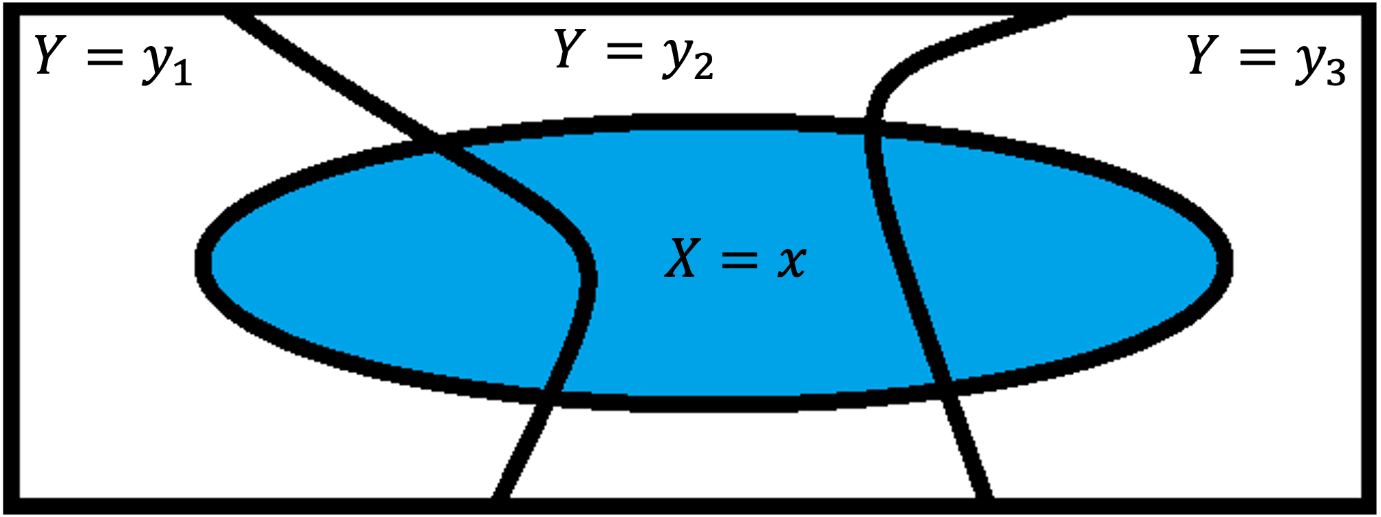
Fig. 5.4 Marginal PMF explained through the Law of Partitions

Example💡: Calculating marginal PMFs from a Joint PMF

Let’s calculate the marginal distributions for the independent fair dice example.

Marginal PMFs from the Joint PMF of for the fair 4-sided and 6-sided dice
\(x \backslash y\)	1	2	3	4	5	6	\(p_X(x)\)
1	\(\tfrac{1}{24}\)	\(\tfrac{1}{24}\)	\(\tfrac{1}{24}\)	\(\tfrac{1}{24}\)	\(\tfrac{1}{24}\)	\(\tfrac{1}{24}\)	\(\tfrac{6}{24}=\tfrac14\)
2	\(\tfrac{1}{24}\)	\(\tfrac{1}{24}\)	\(\tfrac{1}{24}\)	\(\tfrac{1}{24}\)	\(\tfrac{1}{24}\)	\(\tfrac{1}{24}\)	\(\tfrac{6}{24}=\tfrac14\)
3	\(\tfrac{1}{24}\)	\(\tfrac{1}{24}\)	\(\tfrac{1}{24}\)	\(\tfrac{1}{24}\)	\(\tfrac{1}{24}\)	\(\tfrac{1}{24}\)	\(\tfrac{6}{24}=\tfrac14\)
4	\(\tfrac{1}{24}\)	\(\tfrac{1}{24}\)	\(\tfrac{1}{24}\)	\(\tfrac{1}{24}\)	\(\tfrac{1}{24}\)	\(\tfrac{1}{24}\)	\(\tfrac{6}{24}=\tfrac14\)
\(p_Y(y)\)	\(\tfrac{4}{24} =\tfrac16\)	\(\tfrac{4}{24} =\tfrac16\)	\(\tfrac{4}{24} =\tfrac16\)	\(\tfrac{4}{24} =\tfrac16\)	\(\tfrac{4}{24} =\tfrac16\)	\(\tfrac{4}{24} =\tfrac16\)

5.2.3. Independence of Random Variables

Definition

Two discrete random variables \(X\) and \(Y\) are independent if and only if their joint PMF factors as the product of their marginal PMFs for all values in the support. Mathematically, they are independent if and only if

\[p_{X,Y}(x,y) = p_X(x) p_Y(y) \text{ for all } (x,y) \in \text{supp}(X,Y).\]

What Does It Mean?

Independence of random variables \(X\) and \(Y\) means that knowing the value of one provides no information about the value of the other.

With respect to the previously learned concept of independence of two events, this means that any event written in terms of \(X\) is independent of any event expressed in terms of \(Y\).

Example💡: Independence of Two Dice Shown Mathematically

In our dice example, \(X\) and \(Y\) are independent because

\[p_{X,Y}(x,y) = \frac{1}{24} = \frac{1}{4} \times \frac{1}{6} = p_X(x) p_Y(y)\]

for all values of \(x\) and \(y\) in the support.

Be cautious 🛑

Independence is an important property that often simplifies probability calculations. However, its convenient properties should only be used when the idependence of \(X\) and \(Y\) is provided or shown mathematically.

Example💡: When the Dice Constrain Each Other

So far we have relied on independence to keep our calculations simple. But real-world mechanisms often couple random quantities, forcing their outcomes to move together.

Two ordinary six-sided dice are altered so that any roll whose sum is less than 3 or greater than 9 is physically impossible.

Let \(X\) represent the outcome of the first die and \(Y\) the outcome of the second die. The rule \(3 \le X+Y \le 9\) prunes the sample space, but among the allowed pairs, every combination is still equally likely. The table below shows the pruned outcomes as ❌ as well as the probabilities of the possible pairs. Since there are 29 unpruned entries in the table, each possible pair \((x,y)\) gets \(p_{X,Y} (x,y)= 1/29.\)

Joint and marginal PMFs of two dice constraining each other
\(x \backslash y\)	1	2	3	4	5	6	\(p_X(x)\)
1	❌	\(\tfrac{1}{29}\)	\(\tfrac{1}{29}\)	\(\tfrac{1}{29}\)	\(\tfrac{1}{29}\)	\(\tfrac{1}{29}\)	\(\tfrac{5}{29}\)
2	\(\tfrac{1}{29}\)	\(\tfrac{1}{29}\)	\(\tfrac{1}{29}\)	\(\tfrac{1}{29}\)	\(\tfrac{1}{29}\)	\(\tfrac{1}{29}\)	\(\tfrac{6}{29}\)
3	\(\tfrac{1}{29}\)	\(\tfrac{1}{29}\)	\(\tfrac{1}{29}\)	\(\tfrac{1}{29}\)	\(\tfrac{1}{29}\)	\(\tfrac{1}{29}\)	\(\tfrac{6}{29}\)
4	\(\tfrac{1}{29}\)	\(\tfrac{1}{29}\)	\(\tfrac{1}{29}\)	\(\tfrac{1}{29}\)	\(\tfrac{1}{29}\)	❌	\(\tfrac{5}{29}\)
5	\(\tfrac{1}{29}\)	\(\tfrac{1}{29}\)	\(\tfrac{1}{29}\)	\(\tfrac{1}{29}\)	❌	❌	\(\tfrac{4}{29}\)
6	\(\tfrac{1}{29}\)	\(\tfrac{1}{29}\)	\(\tfrac{1}{29}\)	❌	❌	❌	\(\tfrac{3}{29}\)
\(p_Y(y)\)	\(\tfrac{5}{29}\)	\(\tfrac{6}{29}\)	\(\tfrac{6}{29}\)	\(\tfrac{5}{29}\)	\(\tfrac{4}{29}\)	\(\tfrac{3}{29}\)

Both dice are now biased toward lower numbers—a direct result of our sum constraint.

Let us now prove or disprove the independence of \(X\) and \(Y\). If we suspect dependence, it suffices to show that the equation \(p_{X,Y}(x,y) = p_X(x)p_Y(y)\) fails for any single pair. Pick the pair \((x=6,\; y=1)\):

\[p_{X,Y}(6,1) \;=\; \frac{1}{29} \quad\text{but}\quad p_X(6)\,p_Y(1) \;=\; \frac{3}{29} \times \frac{5}{29} \;=\; \frac{15}{29^{2}} \;\neq\; \frac{1}{29}.\]

Since the requirement for independence is \(p_{X,Y}(x,y) = p_X(x)p_Y(y)\) for all possible pairs, \(X\) and \(Y\) has already failed the criterion. Therefore, they are dependent.

A joint distribution can encode constraints (a bounded sum in the previous example) that never appear in the marginals alone. Whenever the joint PMF doesn’t factor, dependence is at play.

5.2.4. Bringing It All Together

Key Takeaways 📝

1. A joint probability mass function specifies the probability of two or more discrete random variables taking on specific values simultaneously.

2. Joint PMFs must satisfy the basic probability axioms: non-negativity and summing to 1 over the entire support.

3. Marginal distributions can be derived from a joint PMF by summing over all possible values of the other variable(s).

4. Random variables are independent if and only if their joint PMF equals the product of their marginal PMFs for all values in the support.

5. When random variables are dependent, their joint distribution contains important information about how they relate to each other that isn’t captured by their marginal distributions alone.

5.2.5. Exercises

These exercises develop your skills in working with joint probability mass functions, deriving marginal distributions, and testing for independence of random variables.

Exercise 1: Extracting Marginal PMFs from a Joint PMF

A software company tracks two metrics for their mobile app: \(X\) = number of crashes per user session (0, 1, or 2) and \(Y\) = user satisfaction rating (1 = low, 2 = medium, 3 = high). Based on data from 1000 sessions, they constructed the following joint PMF:

Table 5.3 Joint PMF for App Performance

Joint PMF \(p_{X,Y}(x,y)\)
\(x \backslash y\)	1 (Low)	2 (Med)	3 (High)	\(p_X(x)\)
0	0.05	0.15	0.40
1	0.10	0.12	0.08
2	0.06	0.03	0.01
\(p_Y(y)\)

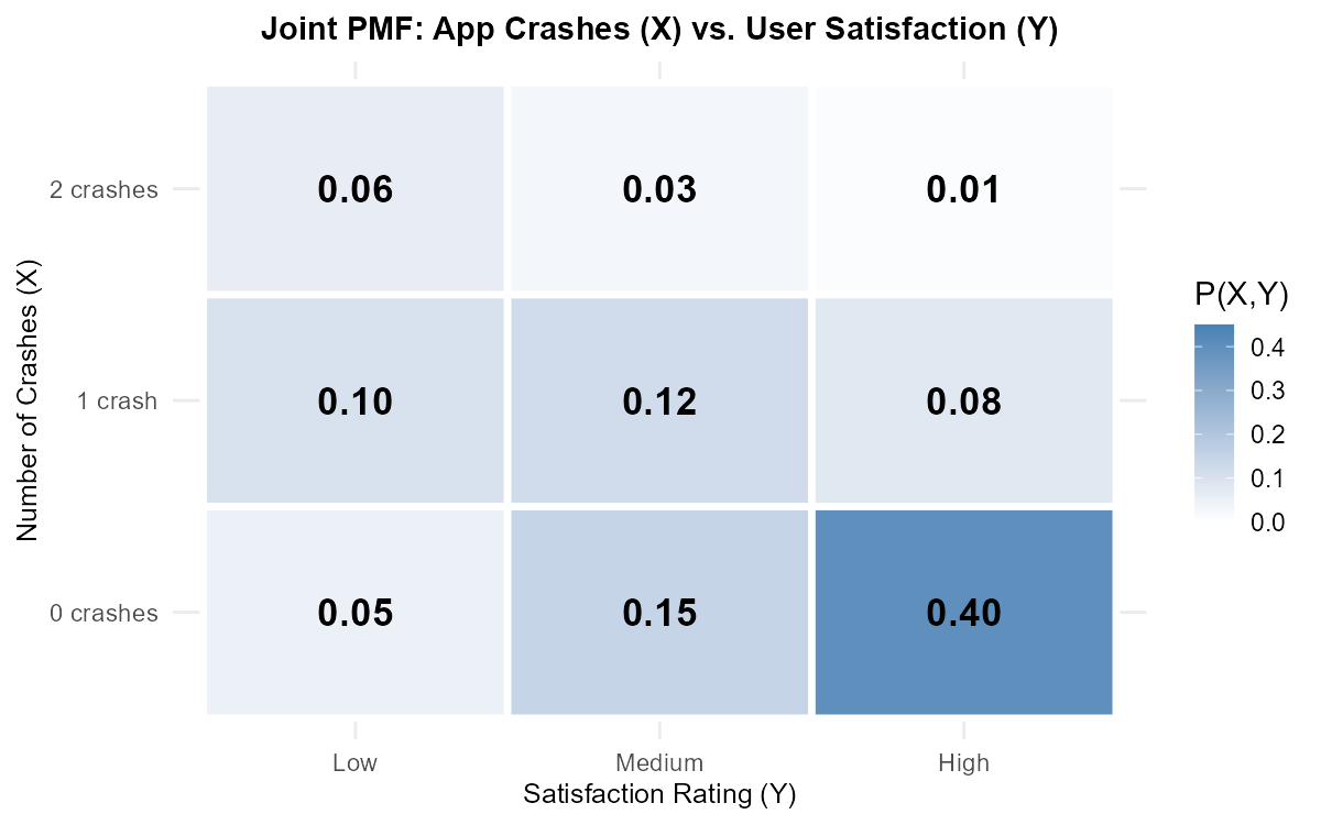
Fig. 5.5 Heatmap visualization of the joint PMF

1. Complete the table by finding the marginal PMFs \(p_X(x)\) and \(p_Y(y)\).

2. Verify that both marginal PMFs are valid.

3. What is the probability that a session has no crashes?

4. What is the probability that a user gives a high satisfaction rating?

5. What is the most likely combination of (crashes, rating)?

Solution

Part (a): Marginal PMFs

Marginal PMF for X (sum across each row):

• \(p_X(0) = 0.05 + 0.15 + 0.40 = 0.60\)

• \(p_X(1) = 0.10 + 0.12 + 0.08 = 0.30\)

• \(p_X(2) = 0.06 + 0.03 + 0.01 = 0.10\)

Marginal PMF for Y (sum down each column):

• \(p_Y(1) = 0.05 + 0.10 + 0.06 = 0.21\)

• \(p_Y(2) = 0.15 + 0.12 + 0.03 = 0.30\)

• \(p_Y(3) = 0.40 + 0.08 + 0.01 = 0.49\)

Completed Table:

Joint PMF \(p_{X,Y}(x,y)\)
\(x \backslash y\)	1 (Low)	2 (Med)	3 (High)	\(p_X(x)\)
0	0.05	0.15	0.40	0.60
1	0.10	0.12	0.08	0.30
2	0.06	0.03	0.01	0.10
\(p_Y(y)\)	0.21	0.30	0.49	1.00

Part (b): Validity Check

For \(p_X(x)\):

• Non-negativity: All values (0.60, 0.30, 0.10) are between 0 and 1 ✓

• Sum: \(0.60 + 0.30 + 0.10 = 1.00\) ✓

For \(p_Y(y)\):

• Non-negativity: All values (0.21, 0.30, 0.49) are between 0 and 1 ✓

• Sum: \(0.21 + 0.30 + 0.49 = 1.00\) ✓

Part (c): P(no crashes)

\(P(X = 0) = p_X(0) = 0.60\)

Part (d): P(high rating)

\(P(Y = 3) = p_Y(3) = 0.49\)

Part (e): Most likely combination

The cell with the highest probability is \(p_{X,Y}(0, 3) = 0.40\).

The most likely combination is (0 crashes, high satisfaction).

---

Exercise 2: Validating a Joint PMF

A network engineer proposes the following joint PMF for two random variables: \(X\) = number of packet errors and \(Y\) = network congestion level.

Table 5.4 Proposed Joint PMF

Joint PMF \(p_{X,Y}(x,y)\)
\(x \backslash y\)	0 (Low)	1 (Med)	2 (High)
0	0.25	0.15	0.05
1	0.10	0.20	0.10
2	0.02	0.08	0.10

1. Verify whether this is a valid joint PMF.

2. If valid, find the marginal PMFs \(p_X(x)\) and \(p_Y(y)\).

3. Calculate \(P(X \leq 1)\).

4. Calculate \(P(X + Y \leq 2)\).

5. Calculate \(P(X = Y)\).

Solution

Part (a): Validity Check

1. Non-negativity: All entries are between 0 and 1 ✓

2. Sum to 1:

   \[\sum_{x,y} p_{X,Y}(x,y) = 0.25 + 0.15 + 0.05 + 0.10 + 0.20 + 0.10 + 0.02 + 0.08 + 0.10 = 1.05\]

   Sum = 1.05 ≠ 1 ✗

This is NOT a valid joint PMF — the probabilities sum to more than 1.

Parts (b)-(e): Since this is not a valid PMF, we cannot meaningfully compute marginal distributions or probabilities. The table would need to be adjusted (e.g., by normalizing) before being used.

Note: In practice, if this arose from data, it might indicate rounding errors. To fix it, we could divide each entry by 1.05 to normalize.

---

Exercise 3: Testing Independence

A quality control process inspects circuit boards on two criteria: \(X\) = number of soldering defects (0 or 1) and \(Y\) = number of component misalignments (0 or 1). The joint PMF is:

Table 5.5 Joint PMF for Circuit Board Defects

Joint PMF \(p_{X,Y}(x,y)\)
\(x \backslash y\)	0	1	\(p_X(x)\)
0	0.70	0.10
1	0.05	0.15
\(p_Y(y)\)

1. Find the marginal PMFs \(p_X(x)\) and \(p_Y(y)\).

2. Determine whether \(X\) and \(Y\) are independent. Show your work.

3. Calculate \(P(X = 1 | Y = 1)\).

4. Compare \(P(X = 1 | Y = 1)\) with \(P(X = 1)\). What does this tell you about the relationship between soldering defects and misalignments?

Solution

Part (a): Marginal PMFs

Marginal for X:

• \(p_X(0) = 0.70 + 0.10 = 0.80\)

• \(p_X(1) = 0.05 + 0.15 = 0.20\)

Marginal for Y:

• \(p_Y(0) = 0.70 + 0.05 = 0.75\)

• \(p_Y(1) = 0.10 + 0.15 = 0.25\)

Part (b): Independence Test

For independence, we need \(p_{X,Y}(x,y) = p_X(x) \cdot p_Y(y)\) for ALL (x,y).

Check each cell:

• \(p_{X,Y}(0,0) = 0.70\) vs \(p_X(0) \cdot p_Y(0) = 0.80 \times 0.75 = 0.60\) → NOT EQUAL

Since the condition fails for (0,0), we can stop here.

X and Y are NOT independent.

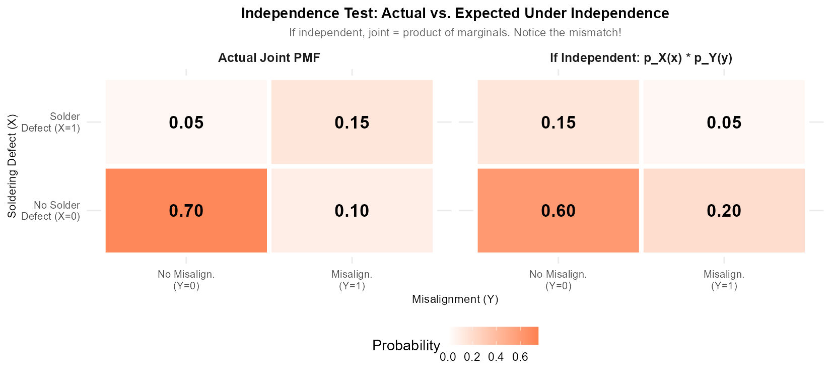
Fig. 5.6 Visual comparison: Actual joint PMF (left) vs. what it would be if X and Y were independent (right)

Verification of other cells (for completeness):

• \(p_{X,Y}(0,1) = 0.10\) vs \(0.80 \times 0.25 = 0.20\) ✗

• \(p_{X,Y}(1,0) = 0.05\) vs \(0.20 \times 0.75 = 0.15\) ✗

• \(p_{X,Y}(1,1) = 0.15\) vs \(0.20 \times 0.25 = 0.05\) ✗

Part (c): Conditional Probability

\[P(X = 1 | Y = 1) = \frac{P(X = 1, Y = 1)}{P(Y = 1)} = \frac{0.15}{0.25} = 0.60\]

Part (d): Interpretation

• \(P(X = 1 | Y = 1) = 0.60\)

• \(P(X = 1) = 0.20\)

When there’s a misalignment (Y = 1), the probability of a soldering defect jumps from 20% to 60%. This strong increase suggests that the two types of defects are positively associated — boards with one type of defect are more likely to have the other.

This could indicate a common cause (e.g., a malfunctioning machine causing both problems) or that one defect makes the other more likely.

---

Exercise 4: Constructing a Joint PMF

A data center monitors two servers. Let \(X\) = number of Server A failures in a day (0 or 1) and \(Y\) = number of Server B failures in a day (0 or 1). Historical data shows:

• Server A fails on 10% of days

• Server B fails on 15% of days

• The servers fail independently of each other

1. Use independence to construct the joint PMF \(p_{X,Y}(x,y)\).

2. What is the probability that at least one server fails on a given day?

3. What is the probability that exactly one server fails?

4. Given that at least one server failed, what is the probability that both failed?

Solution

Part (a): Construct Joint PMF Using Independence

Given:

• \(P(X = 1) = 0.10\), so \(P(X = 0) = 0.90\)

• \(P(Y = 1) = 0.15\), so \(P(Y = 0) = 0.85\)

Since X and Y are independent: \(p_{X,Y}(x,y) = p_X(x) \cdot p_Y(y)\)

\[p_{X,Y}(0,0) = 0.90 \times 0.85 = 0.765\]

\[p_{X,Y}(0,1) = 0.90 \times 0.15 = 0.135\]

\[p_{X,Y}(1,0) = 0.10 \times 0.85 = 0.085\]

\[p_{X,Y}(1,1) = 0.10 \times 0.15 = 0.015\]

Joint PMF Table:

Joint PMF \(p_{X,Y}(x,y)\)
\(x \backslash y\)	0	1	\(p_X(x)\)
0	0.765	0.135	0.90
1	0.085	0.015	0.10
\(p_Y(y)\)	0.85	0.15	1.00

Part (b): P(at least one fails)

“At least one fails” = NOT(both work) = \(1 - P(X=0, Y=0)\)

\[P(X \geq 1 \text{ or } Y \geq 1) = 1 - p_{X,Y}(0,0) = 1 - 0.765 = 0.235\]

Part (c): P(exactly one fails)

“Exactly one” = (A fails, B works) OR (A works, B fails)

\[P(\text{exactly one}) = p_{X,Y}(1,0) + p_{X,Y}(0,1) = 0.085 + 0.135 = 0.220\]

Part (d): P(both failed | at least one failed)

\[P(X=1, Y=1 | X \geq 1 \text{ or } Y \geq 1) = \frac{P(X=1, Y=1)}{P(\text{at least one})} = \frac{0.015}{0.235} \approx 0.0638\]

Given that at least one server failed, there’s about a 6.4% chance both failed.

---

Exercise 5: Joint PMF with Constraints

A manufacturing process produces items that are inspected for defects. Let \(X\) = number of surface defects and \(Y\) = number of internal defects. Due to the inspection process, the total number of detected defects \(X + Y\) is always at most 3.

The joint PMF is given by:

\[p_{X,Y}(x,y) = \frac{c}{(x+y+1)} \quad \text{for } x, y \in \{0, 1, 2\} \text{ and } x + y \leq 3\]

where \(c\) is a normalizing constant.

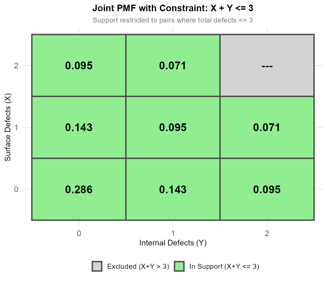
Fig. 5.7 The constraint X + Y ≤ 3 creates an irregular support (green = valid, gray = excluded)

1. List all pairs (x, y) in the support of this joint PMF.

2. Find the value of \(c\) that makes this a valid PMF.

3. Construct the joint PMF table.

4. Find the marginal PMF \(p_X(x)\).

5. Are X and Y independent? Justify your answer.

Solution

Part (a): Support

We need \(x, y \in \{0, 1, 2\}\) and \(x + y \leq 3\).

Valid pairs:

• x = 0: (0,0), (0,1), (0,2) — all satisfy x + y ≤ 3

• x = 1: (1,0), (1,1), (1,2) — all satisfy x + y ≤ 3

• x = 2: (2,0), (2,1) — (2,2) would give x + y = 4 > 3, excluded

Support: {(0,0), (0,1), (0,2), (1,0), (1,1), (1,2), (2,0), (2,1)}

Part (b): Finding c

Sum over all pairs in support:

\[\sum_{(x,y)} \frac{c}{x+y+1} = c\left(\frac{1}{1} + \frac{1}{2} + \frac{1}{3} + \frac{1}{2} + \frac{1}{3} + \frac{1}{4} + \frac{1}{3} + \frac{1}{4}\right)\]

\[= c\left(1 + \frac{1}{2} + \frac{1}{2} + \frac{1}{3} + \frac{1}{3} + \frac{1}{3} + \frac{1}{4} + \frac{1}{4}\right)\]

\[= c\left(1 + 1 + 1 + \frac{1}{2}\right) = c \times \frac{7}{2} = \frac{7c}{2}\]

For validity: \(\frac{7c}{2} = 1 \implies c = \frac{2}{7}\)

Part (c): Joint PMF Table

Using \(p_{X,Y}(x,y) = \frac{2}{7(x+y+1)}\):

Joint PMF \(p_{X,Y}(x,y)\)
\(x \backslash y\)	0	1	2	\(p_X(x)\)
0	\(\frac{2}{7}\)	\(\frac{1}{7}\)	\(\frac{2}{21}\)	\(\frac{11}{21}\)
1	\(\frac{1}{7}\)	\(\frac{2}{21}\)	\(\frac{1}{14}\)	\(\frac{13}{42}\)
2	\(\frac{2}{21}\)	\(\frac{1}{14}\)	—	\(\frac{7}{42} = \frac{1}{6}\)
\(p_Y(y)\)	\(\frac{11}{21}\)	\(\frac{13}{42}\)	\(\frac{1}{6}\)	1

Part (d): Marginal PMF for X

• \(p_X(0) = \frac{2}{7} + \frac{1}{7} + \frac{2}{21} = \frac{6}{21} + \frac{3}{21} + \frac{2}{21} = \frac{11}{21}\)

• \(p_X(1) = \frac{1}{7} + \frac{2}{21} + \frac{1}{14} = \frac{6}{42} + \frac{4}{42} + \frac{3}{42} = \frac{13}{42}\)

• \(p_X(2) = \frac{2}{21} + \frac{1}{14} = \frac{4}{42} + \frac{3}{42} = \frac{7}{42} = \frac{1}{6}\)

Check: \(\frac{11}{21} + \frac{13}{42} + \frac{1}{6} = \frac{22}{42} + \frac{13}{42} + \frac{7}{42} = \frac{42}{42} = 1\) ✓

Part (e): Independence Test

Check if \(p_{X,Y}(0,0) = p_X(0) \cdot p_Y(0)\):

• \(p_{X,Y}(0,0) = \frac{2}{7}\)

• \(p_X(0) \cdot p_Y(0) = \frac{11}{21} \times \frac{11}{21} = \frac{121}{441}\)

Convert \(\frac{2}{7} = \frac{126}{441}\)

Since \(\frac{126}{441} \neq \frac{121}{441}\), X and Y are NOT independent.

The constraint \(x + y \leq 3\) creates dependence — knowing X limits the possible values of Y.

---

Exercise 6: Working with a Given Joint PMF

Two sensors monitor temperature (X) and humidity (Y) in a data center, where both are discretized into levels 1, 2, or 3. The joint PMF is:

Table 5.6 Joint PMF for Sensor Readings

Joint PMF \(p_{X,Y}(x,y)\)
\(x \backslash y\)	1	2	3	\(p_X(x)\)
1	0.15	0.10	0.05	0.30
2	0.10	0.25	0.10	0.45
3	0.05	0.10	0.10	0.25
\(p_Y(y)\)	0.30	0.45	0.25	1.00

1. Calculate \(P(X \leq 2, Y \leq 2)\).

2. Calculate \(P(X = Y)\).

3. Calculate \(P(X < Y)\).

4. Calculate \(P(Y = 2 | X = 2)\).

5. Calculate \(P(X \geq 2 | Y \leq 2)\).

6. Are X and Y independent?

Solution

Part (a): P(X ≤ 2, Y ≤ 2)

Sum all cells where x ≤ 2 AND y ≤ 2:

\[P(X \leq 2, Y \leq 2) = p_{X,Y}(1,1) + p_{X,Y}(1,2) + p_{X,Y}(2,1) + p_{X,Y}(2,2)\]

\[= 0.15 + 0.10 + 0.10 + 0.25 = 0.60\]

Part (b): P(X = Y)

Sum diagonal cells where x = y:

\[P(X = Y) = p_{X,Y}(1,1) + p_{X,Y}(2,2) + p_{X,Y}(3,3)\]

\[= 0.15 + 0.25 + 0.10 = 0.50\]

Part (c): P(X < Y)

Sum cells where x < y (below the diagonal):

\[P(X < Y) = p_{X,Y}(1,2) + p_{X,Y}(1,3) + p_{X,Y}(2,3)\]

\[= 0.10 + 0.05 + 0.10 = 0.25\]

Part (d): P(Y = 2 | X = 2)

\[P(Y = 2 | X = 2) = \frac{P(X = 2, Y = 2)}{P(X = 2)} = \frac{0.25}{0.45} = \frac{5}{9} \approx 0.556\]

Part (e): P(X ≥ 2 | Y ≤ 2)

First, find \(P(X \geq 2, Y \leq 2)\):

\[P(X \geq 2, Y \leq 2) = p_{X,Y}(2,1) + p_{X,Y}(2,2) + p_{X,Y}(3,1) + p_{X,Y}(3,2)\]

\[= 0.10 + 0.25 + 0.05 + 0.10 = 0.50\]

Then:

\[P(Y \leq 2) = p_Y(1) + p_Y(2) = 0.30 + 0.45 = 0.75\]

\[P(X \geq 2 | Y \leq 2) = \frac{P(X \geq 2, Y \leq 2)}{P(Y \leq 2)} = \frac{0.50}{0.75} = \frac{2}{3} \approx 0.667\]

Part (f): Independence Test

Check one cell: \(p_{X,Y}(1,1) = 0.15\)

\(p_X(1) \cdot p_Y(1) = 0.30 \times 0.30 = 0.09\)

Since \(0.15 \neq 0.09\), X and Y are NOT independent.

---

5.2.6. Additional Practice Problems

True/False Questions (1 point each)

1. A joint PMF \(p_{X,Y}(x,y)\) gives the probability that X equals x OR Y equals y.

   Ⓣ or Ⓕ

2. The marginal PMF \(p_X(x)\) is found by summing the joint PMF over all values of Y.

   Ⓣ or Ⓕ

3. If X and Y are independent, then \(p_{X,Y}(x,y) = p_X(x) + p_Y(y)\).

   Ⓣ or Ⓕ

4. All entries in a valid joint PMF must be non-negative.

   Ⓣ or Ⓕ

5. If \(p_{X,Y}(1,2) = p_X(1) \cdot p_Y(2)\), then X and Y are independent.

   Ⓣ or Ⓕ

6. The sum of all entries in a joint PMF table must equal 1.

   Ⓣ or Ⓕ

Multiple Choice Questions (2 points each)

7. Given the joint PMF below, what is \(p_X(1)\)?

   \(x \backslash y\)	0	1	2
   0	0.1	0.2	0.1
   1	0.15	0.25	0.2

   Ⓐ 0.25

   Ⓑ 0.45

   Ⓒ 0.60

   Ⓓ 0.40

8. Using the joint PMF from Question 7, what is \(P(X = Y)\)?

   Ⓐ 0.10

   Ⓑ 0.35

   Ⓒ 0.45

   Ⓓ 0.55

9. If X and Y are independent with \(P(X = 0) = 0.6\) and \(P(Y = 1) = 0.3\), what is \(P(X = 0, Y = 1)\)?

   Ⓐ 0.90

   Ⓑ 0.30

   Ⓒ 0.18

   Ⓓ 0.50

10. Which of the following is necessary for X and Y to be independent?

    Ⓐ \(p_{X,Y}(x,y) = p_X(x) \cdot p_Y(y)\) for at least one pair (x,y)

    Ⓑ \(p_{X,Y}(x,y) = p_X(x) \cdot p_Y(y)\) for all pairs (x,y) in the support

    Ⓒ \(p_{X,Y}(x,y) = p_X(x) + p_Y(y)\) for all pairs (x,y)

    Ⓓ \(P(X = Y) = 0\)

Answers to Practice Problems

True/False Answers:

1. False — A joint PMF gives the probability that X equals x AND Y equals y simultaneously, not OR.

2. True — By definition, \(p_X(x) = \sum_y p_{X,Y}(x,y)\). This is summing over all possible values of Y for each fixed x.

3. False — If independent, \(p_{X,Y}(x,y) = p_X(x) \cdot p_Y(y)\) (product, not sum).

4. True — Non-negativity is one of the two axioms for a valid joint PMF: \(0 \leq p_{X,Y}(x,y) \leq 1\) for all (x,y).

5. False — Independence requires the product formula to hold for ALL pairs (x,y) in the support, not just one pair.

6. True — The second axiom for validity: \(\sum_{(x,y)} p_{X,Y}(x,y) = 1\).

Multiple Choice Answers:

7. Ⓒ — \(p_X(1) = 0.15 + 0.25 + 0.20 = 0.60\) (sum of row where x = 1).

8. Ⓑ — \(P(X = Y)\) = \(p_{X,Y}(0,0) + p_{X,Y}(1,1) = 0.10 + 0.25 = 0.35\). Note: (0,0) is in the support; there’s no (2,2) entry for x.

9. Ⓒ — By independence: \(P(X = 0, Y = 1) = P(X = 0) \cdot P(Y = 1) = 0.6 \times 0.3 = 0.18\).

10. Ⓑ — Independence requires the product formula to hold for all pairs in the support, not just some.