Slides 📊

Download Chapter 6 slides (PPTX)

6.3. Cumulative Distribution Functions

Computing probabilities for continuous random variables requires integrating the PDF over intervals, which can become tedious when we need to calculate many different probabilities. Just as calculus provides us with antiderivatives to avoid repeated integration, probability theory offers us the cumulative distribution function (CDF) as a tool that eliminates the need for repeated integrations.

Road Map 🧭

• Define the cumulative distribution function (CDF).

• Master the relationship between PDF and CDF through the fundamental theorem of calculus.

• Learn the essential properties of CDFs that make them valid probability functions.

• Practice computing probabilities using CDFs instead of direct integration.

• Apply CDFs to find percentiles and quantiles for continuous distributions.

6.3.1. The Universal Language of Cumulative Probability

The cumulative distribution function (CDF) provides a unified approach to probability that works seamlessly for both discrete and continuous random variables. Instead of dealing with probability mass functions and probability density functions separately, the CDF gives us one consistent framework.

Definition

For any random variable \(X\) (discrete or continuous), the cumulative distribution function \(F_X(x)\) is defined as:

\[F_X(x) = P(X \leq x)\]

The definition expresses a simple idea: \(F_X(x)\) gives the probability that the random variable \(X\) falls at or below any given value \(x\).

Implementation of CDF to Different Variable Types
Discrete	Continuous
\[F_X(x) = P(X \leq x) = \sum_{t=-\infty}^{x} p_X(t)\]	\[F_X(x) = P(X \leq x) = \int_{-\infty}^{x} f_X(t) \, dt\]

In both cases, the argument of the PMF/PDF is replaced with a dummy variable \(t\). This is to avoid any confusion with the true argument of \(F_X\).

In the continuous case, \(F_X(x)\) can be used for \(P(X\leq x)\) or \(P(X<x)\).

6.3.2. Requirements for a valid CDF

Cumulative distribution functions must satisfy several mathematical properties that reflect their probabilistic interpretation.

1. Monotonicity

As we move from a smaller to a larger \(x\), we can only accumulate the probability that \(X\) falls below it. Therefore, \(F_X\) is a non-decreasing function. That is, for any real numbers \(a < b\),

\[F_X(a) \leq F_X(b)\]

2. Limiting Behavior

The accumulated probability must be close to 0 at a very small \(x\) (no probability accumulates infinitely far to the left on the x-axis), and close to 1 for a large enough \(x\):

\[\lim_{x \to -\infty} F_X(x) = 0 \quad \text{and} \quad \lim_{x \to +\infty} F_X(x) = 1\]

3: Right Continuity

For any point \(c\),

\[\lim_{x \to c^+} F_X(x) = F_X(c).\]

This technical property ensures that the CDF behaves consistently at boundary points, particularly important when dealing with mixed discrete-continuous distributions or piecewise functions. This property is satisfied automatically for continuous distributions.

6.3.3. The PDF-CDF Connection

For continuous random variables, the relationship between a PDF and its CDF mirrors the fundamental theorem of calculus.

From PDF to CDF: Integration

By the definition,

\[F_X(x) = \int_{-\infty}^{x} f_X(t) \, dt\]

\(F_X(x)\) is the accummulation of all the probability from the left tail of the distribution up to the point \(x\).

From CDF to PDF: Differentiation

Given a CDF \(F_X(x)\), we can recover the PDF by differentiation:

\[f_X(x) = \frac{d}{dx} F_X(x) = F_X'(x)\]

wherever the derivative exists. This relationship explains why the PDF measures the “rate of accumulation” of probability at each point.

Visualizing the Relationship

The connection becomes clear when we graph the two functions together.

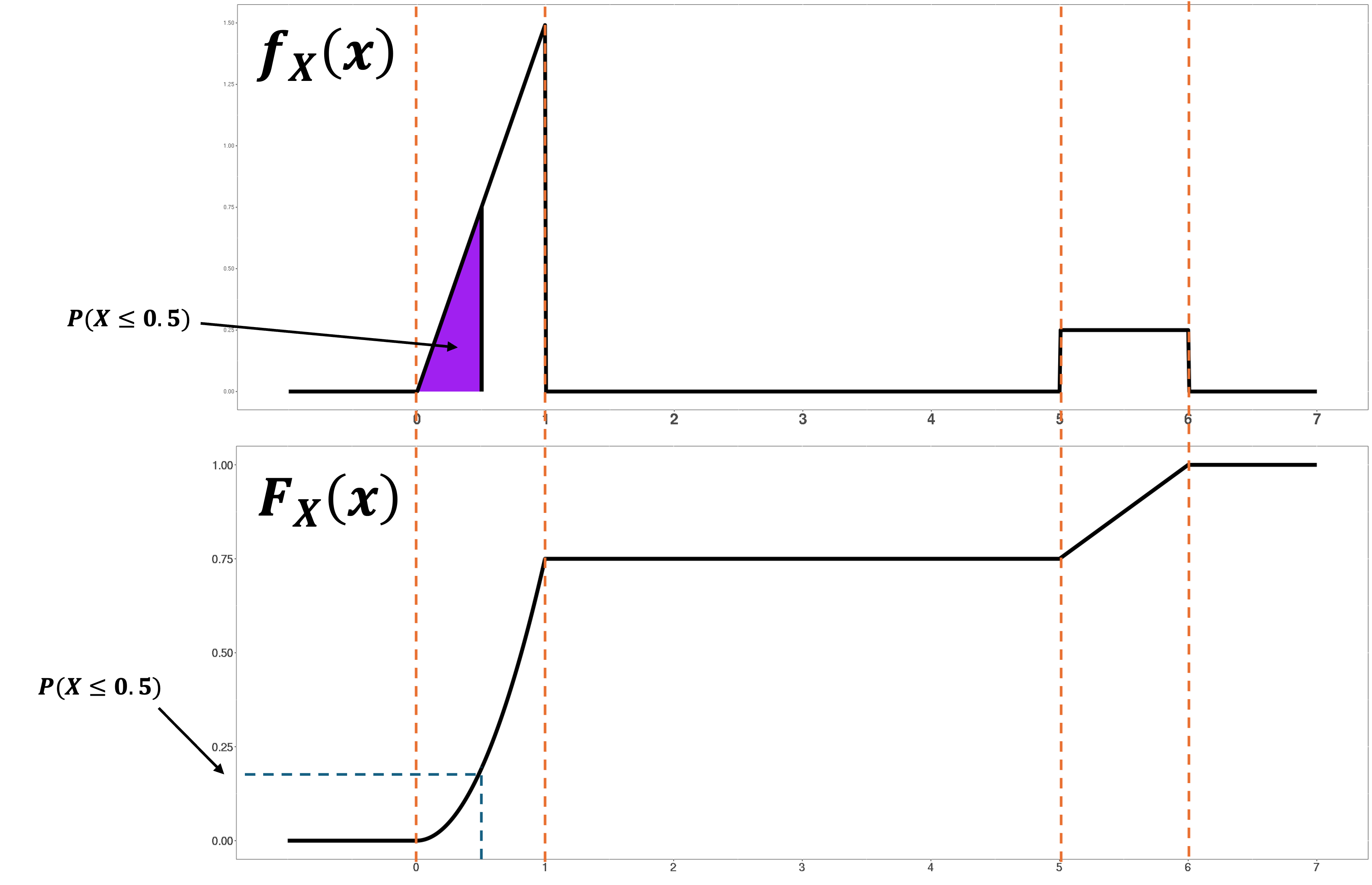
Fig. 6.15 Relationship between PDF and CDF

• If one function is piecewise-defined, the other is as well. They share the same set of boundaries.

• A probability of the form \(P(X\leq a)\) corresponds to the area to the left of \(a\) under a PDF, and to the height of the curve on a CDF.

• A PDF can take any shape, as long as it stays above the horizontal axis and integrates to 1. A CDF is more constrained in shape; it approaches 0 on the left, 1 on the right, and is never decreasing in between.

• In any region where the PDF is \(0\), the CDF is flat, but not necessarily 0. It retains any area accummulated in previous regions, but no area accummulates additionally.

6.3.4. Building a Piecewise CDF

Constructing a CDF based on a piecewise-defined PDF requires careful attention. The most crucial aspect of working with piecewise CDFs is remembering that they are cumulative—they must account for all probability accumulated up to each point, not just in the current region.

Useful tips for constructing a piecewise CDF:

• Make a rough sketch similar to Fig. 6.15. Visually identify the regions where the CDF is approaching 0, incresing, flat, or approaching 1. At the end, check whether the computational result matches the sketch.

• Stick to the definition at first. By definition,

  \[F_X(x) = \int_{-\infty}^x f_X(t) \, dt\]

  is an integral from negative infinity up to the input value, \(x\). Starting directly from this definition—without skipping steps—will help you become familiar with the subtle patterns involved in constructing piecewise CDFs.

Example💡: Constructing the CDF for a piecewise PDF

Construct the CDF of a random variable \(X\) which has the following PDF. Use Fig. 6.15 as reference.

\[\begin{split}f_X(x) = \begin{cases} \frac{3x}{2} & \text{for } 0 \leq x \leq 1 \\ 0 & \text{for } 1 < x < 5 \\ \frac{1}{4} & \text{for } 5 \leq x \leq 6 \\ 0 & \text{elsewhere} \end{cases}\end{split}\]

Work on each region given by the PDF separately:

Region 1 (\(x < 0\)): No probability accumulated yet

\[F_X(x) = \int_{-\infty}^x f_X(t) \, dt = \int_{-\infty}^x 0 \, dt = 0\]

Region 2 (\(0 \leq x \leq 1\)): Accumulating triangular area

\[F_X(x) = \int_{-\infty}^x f_X(t) \, dt = \underbrace{\int_{-\infty}^0 f_X(t)dt}_{=F_X(0) = 0} + \int_0^x \frac{3t}{2} \, dt = \frac{3x^2}{4}\]

Region 3 (\(1 < x < 5\)): No new probability, but keep previous accumulation

\[\begin{split}F_X(x) &= \int_{-\infty}^x f_X(t) \, dt \\ &= \underbrace{\int_{-\infty}^0 f_X(t)dt + \int_0^1 \frac{3t}{2} \, dt}_{=F_X(1) = \frac{3}{4}} + \underbrace{\int_1^x f_X(t) \, dt}_{=0} = \frac{3}{4}\end{split}\]

The area is constant at the triangle’s total area.

Region 4 (\(5 \leq x \leq 6\)): Add rectangular area to previous accumulation

\[\begin{split}F_X(x) &= \int_{-\infty}^x f_X(t) \, dt \\ &= \underbrace{\int_{-\infty}^0 f_X(t)dt + \int_0^1 \frac{3t}{2} \, dt + \int_1^5 f_X(t) \, dt}_{=F_X(5)=\frac{3}{4}} + \int_5^x f_X(t) \, dt\\ &=\frac{3}{4} + \int_5^x \frac{1}{4} \, dt = \frac{3}{4} + \frac{x-5}{4} = \frac{x-2}{4}\end{split}\]

Region 5 (\(x > 6\)): All probability has been accumulated

\[\begin{split}F_X(x) &= \int_{-\infty}^x f_X(t) \, dt \\ &= F_X(6) + \int_{6}^{\infty} f_X(t) \, dt = 1 + \int_6^{\infty} 0 \, dt = 1.\end{split}\]

Putting together,

\[\begin{split}F_X(x) = \begin{cases} 0 & \text{for } x < 0 \\ \frac{3x^2}{4} & \text{for } 0 \leq x \leq 1 \\ \frac{3}{4} & \text{for } 1 < x < 5 \\ \frac{x-2}{4} & \text{for } 5 \leq x \leq 6 \\ 1 & \text{for } x > 6 \end{cases}\end{split}\]

• The video below goes through the series of examples covered in this section.

🛑 Know how to avoid the common mistake before simplifying steps

In all regions beyond the first in the previous example, the CDF \(f_X(x)\) is computed as the sum of area accumulated in the earlier regions plus the integral over the current region.

Forgetting to factor in the area from previous regions is a very common mistake made by students. While you may eventually skip some redundant steps as you gain familiarity, your top priority should be to avoid this error.

6.3.5. Computing Probabilities with CDFs

Once we have the CDF, calculating probabilities becomes remarkably straightforward. We can handle any probability problems without additional integration.

Recall that equality signs do not matter for continuous RVs

All the rules below will apply if \(<\) and \(\leq\) are interchanged as well as if \(>\) and \(\geq\) are switched because \(P(X = a) = 0\) for any single point \(a\).

Basic CDF Evaluation

For \(P(X \leq a)\),

\[P(X \leq a) = F_X(a)\]

This is just the definition of the CDF—plug in the value and read the result.

“Greater Than” Probabilities

For \(P(X > a)\), we use the complement rule:

\[P(X > a) = 1 - P(X \leq a) = 1 - F_X(a)\]

The probability of exceeding \(a\) equals one minus the probability of not exceeding \(a\).

Interval Probabilities

For \(P(a < X \leq b)\), we take the accumulated probability up to \(b\) and subtract the accumulated probability up to \(a\), leaving just the probability in the interval.

\[P(a < X \leq b) = F_X(b) - F_X(a)\]

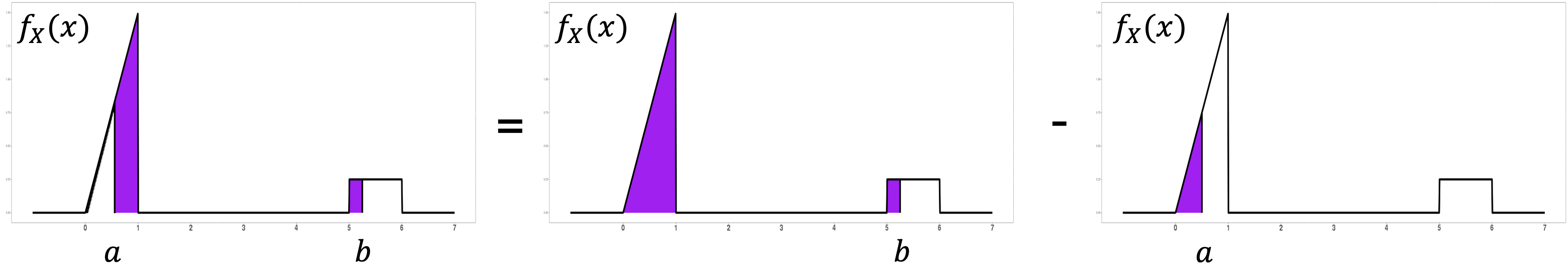
Fig. 6.16 P(a < X ≤ b) equals the difference between CDF values

Example💡: Computing Probabilities Using a CDF

Use the PDF and CDF found in the previous example to answer the questions below.

\[\begin{split}f_X(x) = \begin{cases} \frac{3x}{2} & \text{for } 0 \leq x \leq 1 \\ \frac{1}{4} & \text{for } 5 \leq x \leq 6 \\ 0 & \text{elsewhere} \end{cases}\end{split}\]

\[\begin{split}F_X(x) = \begin{cases} 0 & \text{for } x < 0 \\ \frac{3x^2}{4} & \text{for } 0 \leq x < 1 \\ \frac{3}{4} & \text{for } 1 \leq x < 5 \\ \frac{x-2}{4} & \text{for } 5 \leq x \leq 6 \\ 1 & \text{for } x > 6 \end{cases}\end{split}\]

1. Find \(P(X \leq 0.5)\).

   \(x=0.5\) belongs to Region 2 of the CDF, so \(F_X(0.5) = \frac{3(0.5)^2}{4} = \frac{3}{16}\).

2. Find \(P(X \geq 5.5)\).

   \(P(X \geq 5.5) = 1 - P(X < 5.5) = 1 - F_X(5.5)\). \(x=5.5\) is in Region 4. Therefore, \(P(X > 5.5) = 1 - \frac{5.5-2}{4} = 1 - \frac{7}{8} = \frac{1}{8}\)

3. Find \(P(0.2 < X \leq 5.8)\).

   \[\begin{split}P(0.2 < X \leq 5.8) &= F_X(5.8) - F_X(0.2) = \frac{5.8-2}{4} -\frac{3(0.2)^2}{4}\\ &= 0.95 - 0.03 = 0.92.\end{split}\]

6.3.6. Finding Percentiles using CDF

Definition

Take a value \(p \in [0,1]\). The \(p \times 100\) th percentile of a random variable \(X\), denoted \(x_p\), is the value satisfying:

\[F_X(x_p) = P(X \leq x_p) = p.\]

For example,

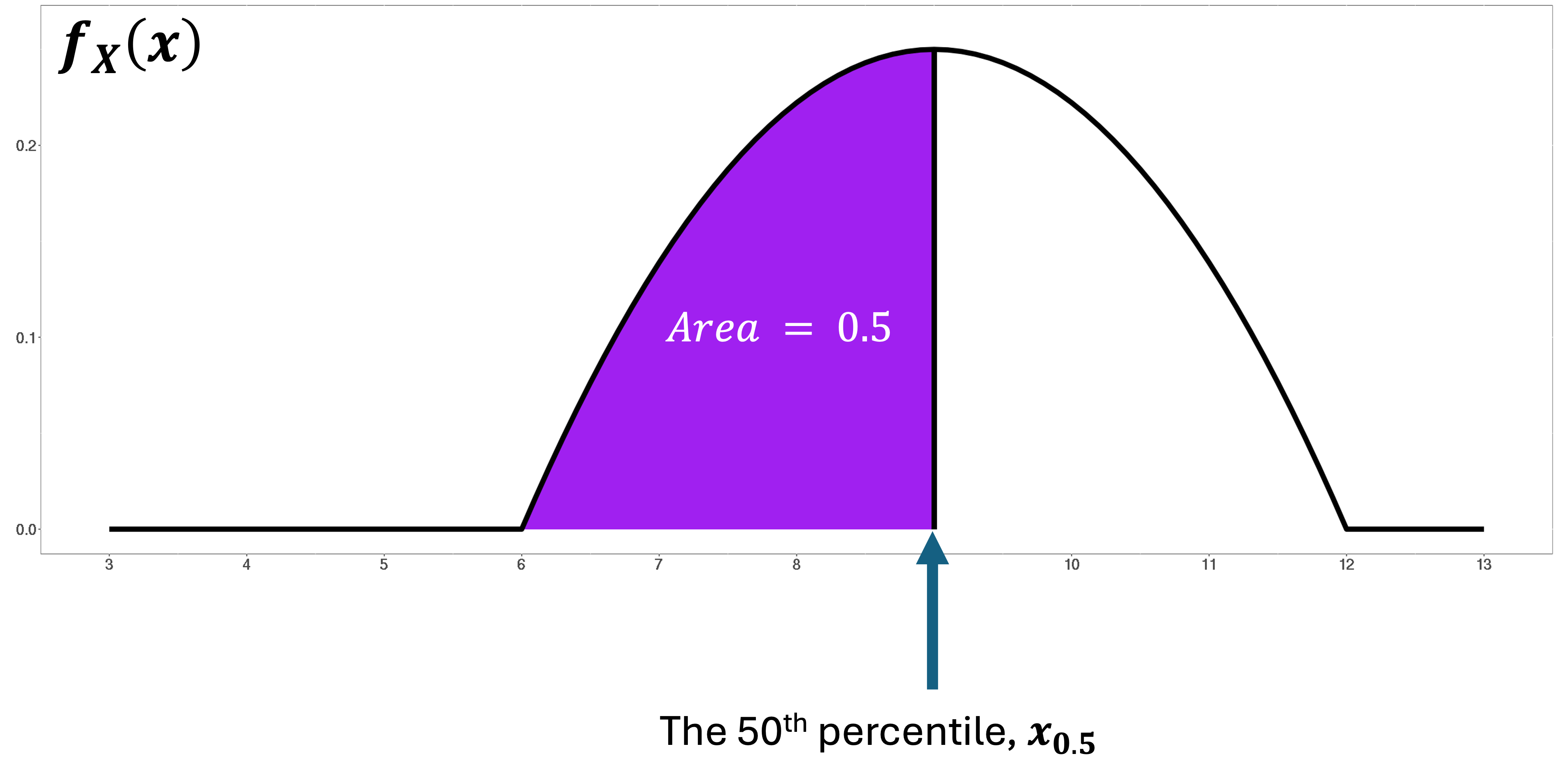
• The 50th percentile of a random variable \(X\) is written as \(x_{0.5}\) and satisfies the conditon:

  \[F_X(x_{0.5}) = P(X \leq x_{0.5})= 0.5.\]

  \(x_{0.5}\) represents the vertical cutoff on the PDF of \(X\) such that the area to its left is exactly \(0.5\). This special percentile is also called the median (\(\tilde{\mu}\)) of \(X\).

  

• The 25th percentile \(x_{0.25}\) satisfies \(F_X(x_{0.25}) = 0.25\). It splits the PDF into a left region with area 0.25 and right region with area 0.75.

• The 75th percentile \(x_{0.75}\) satisfies \(F_X(x_{0.75}) = 0.75\). It splits the PDF into a left region with area 0.75 and right region with area 0.25.

• The true IQR of \(X\) is the difference of \(x_{0.75} - x_{0.25}\).

Connection to sample percentiles

Recall that we’ve already discussed the concept of sample percentiles for a dataset in Chapter 3. The percentiles for a random variable are considered their population equivalent in the framework of data analysis.

If we generate data points \(x_1, x_2,\cdots, x_n\) from a random variable \(X\), we would compute the sample percentiles using \(x_1, x_2,\cdots, x_n\), and the true percentiles using the CDF of \(X\). The two sets of objects are closely related, but different.

Computing Percentiles of a Continuous Random Variable

Percentiles for a continuous random variables are found by replacing the general definition \(F_X(x_p) = p\) with specific expressions, than solving for \(x_p\). See the example below for further detail.

Example💡: Finding a Percentile

Find the 85th percentile of a random variable \(X\) which has the following CDF:

\[\begin{split}F_X(x) = \begin{cases} 0 & \text{for } x < 0 \\ \frac{3x^2}{4} & \text{for } 0 \leq x < 1 \\ \frac{3}{4} & \text{for } 1 \leq x < 5 \\ \frac{x-2}{4} & \text{for } 5 \leq x \leq 6 \\ 1 & \text{for } x > 6 \end{cases}\end{split}\]

We must solve \(F_X(x_{0.85}) = 0.85\) for \(x_{0.85}\).

Which piece of the CDF should we use to replace the general expression \(F_X(x_{0.85})\)? Since \(F_X(5) = \frac{3}{4} = 0.75 < 0.85\), we know that the 85th percentile has to be strictly greater than \(5\). Using Region 4,

\[\begin{split}&\frac{x_{0.85} - 2}{4} = 0.85\\ &x_{0.85} - 2 = 3.4\\ &x_{0.85} = 5.4\end{split}\]

6.3.7. More examples

6.3.8. Bringing It All Together

Key Takeaways 📝

1. The cumulative distribution function \(F_X(x) = P(X \leq x)\) provides a universal framework for both discrete and continuous random variables. It eliminates the need for repeated integration when computing probabilities for continuous random variables.

2. For continuous variables, PDFs and CDFs are related through differentiation and integration: \(f_X(x) = F_X'(x)\) and \(F_X(x) = \int_{-\infty}^x f_X(t) \, dt\).

3. Valid CDFs must be non-decreasing, approach 0 as \(x \to -\infty\), approach 1 as \(x \to +\infty\), and be right-continuous.

4. Probability calculations become simpler with CDFs: \(P(X \leq a) = F_X(a)\), \(P(X > a) = 1 - F_X(a)\), and \(P(a < X \leq b) = F_X(b) - F_X(a)\).

5. Piecewise CDFs require careful attention—each region must include all probability accumulated from previous regions.

6. Percentiles are found by solving \(F_X(x_p) = p\).

In our next sections, we’ll see how these concepts apply to specific named distributions, starting with the most important continuous distribution in all of statistics: the normal distribution.

6.3.9. Exercises

These exercises develop your skills in constructing cumulative distribution functions, computing probabilities using CDFs, finding percentiles, and understanding the PDF-CDF relationship.

Reminder

For continuous random variables, \(P(X = a) = 0\) for any single point \(a\). This means strict and non-strict inequalities give the same probability: \(P(X < a) = P(X \leq a)\) and \(P(X > a) = P(X \geq a)\). Throughout these exercises, we use whichever form is convenient.

Exercise 1: Basic CDF Construction

A quality control engineer models the thickness \(X\) (in mm) of a protective coating with PDF:

\[\begin{split}f_X(x) = \begin{cases} 2x, & 0 \leq x \leq 1\\ 0, & \text{elsewhere} \end{cases}\end{split}\]

1. Construct the CDF \(F_X(x)\) for all regions.

2. Verify that your CDF satisfies all three required properties: monotonicity, limiting behavior, and right-continuity.

3. Use the CDF to find \(P(X \leq 0.6)\).

4. Use the CDF to find \(P(X > 0.7)\).

5. Use the CDF to find \(P(0.3 < X \leq 0.8)\).

6. Find the median coating thickness.

Solution

Part (a): Construct the CDF

Region 1 (\(x < 0\)): No probability accumulated yet.

\[F_X(x) = \int_{-\infty}^{x} f_X(t) \, dt = \int_{-\infty}^{x} 0 \, dt = 0\]

Region 2 (\(0 \leq x \leq 1\)): Accumulate probability from the start of support.

\[F_X(x) = \int_{-\infty}^{x} f_X(t) \, dt = \underbrace{\int_{-\infty}^{0} 0 \, dt}_{=0} + \int_{0}^{x} 2t \, dt = t^2 \Big|_0^x = x^2\]

Region 3 (\(x > 1\)): All probability accumulated.

\[F_X(x) = F_X(1) + \int_{1}^{x} 0 \, dt = 1 + 0 = 1\]

Complete CDF:

\[\begin{split}F_X(x) = \begin{cases} 0, & x < 0\\ x^2, & 0 \leq x \leq 1\\ 1, & x > 1 \end{cases}\end{split}\]

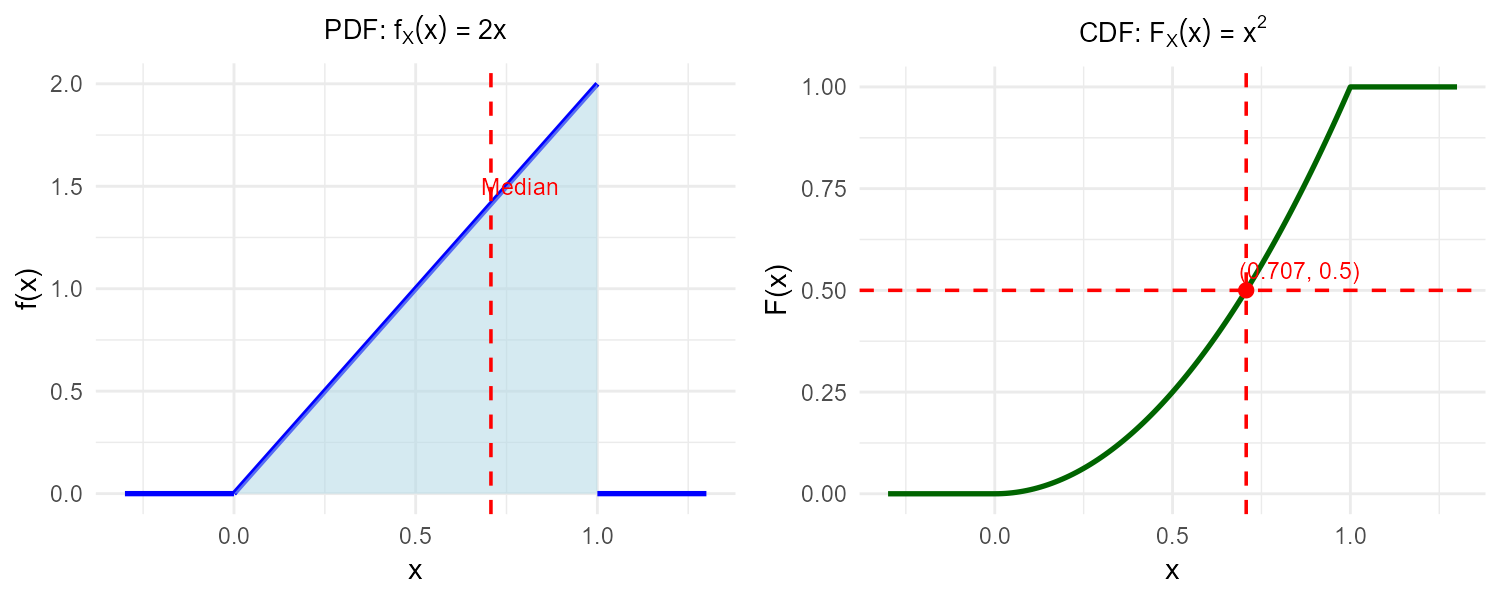
Fig. 6.17 Left: PDF \(f_X(x) = 2x\). Right: CDF \(F_X(x) = x^2\) on [0,1].

Part (b): Verify CDF properties

1. Monotonicity: On \([0, 1]\), \(F_X(x) = x^2\) has derivative \(F_X'(x) = 2x \geq 0\), so it’s non-decreasing. The function is constant (0 or 1) outside this interval. ✓

2. Limiting behavior:

• \(\lim_{x \to -\infty} F_X(x) = 0\) ✓

• \(\lim_{x \to +\infty} F_X(x) = 1\) ✓

3. Right-continuity: The function is continuous everywhere (no jumps), so right-continuity is satisfied automatically. ✓

Part (c): P(X ≤ 0.6)

\[P(X \leq 0.6) = F_X(0.6) = (0.6)^2 = 0.36\]

Part (d): P(X > 0.7)

\[P(X > 0.7) = 1 - P(X \leq 0.7) = 1 - F_X(0.7) = 1 - (0.7)^2 = 1 - 0.49 = 0.51\]

Part (e): P(0.3 < X ≤ 0.8)

\[P(0.3 < X \leq 0.8) = F_X(0.8) - F_X(0.3) = (0.8)^2 - (0.3)^2 = 0.64 - 0.09 = 0.55\]

Part (f): Median

Solve \(F_X(x_{0.5}) = 0.5\):

\[x_{0.5}^2 = 0.5 \implies x_{0.5} = \sqrt{0.5} = \frac{1}{\sqrt{2}} \approx 0.707 \text{ mm}\]

---

Exercise 2: CDF with Non-Zero Starting Point

A biomedical engineer models drug concentration \(X\) (in mg/L) in the bloodstream with PDF:

\[\begin{split}f_X(x) = \begin{cases} \frac{1}{2}(x - 2), & 2 \leq x \leq 4\\ 0, & \text{elsewhere} \end{cases}\end{split}\]

Note that the support starts at \(x = 2\), not \(x = 0\).

1. Verify this is a valid PDF.

2. Construct the complete CDF \(F_X(x)\).

3. Find \(P(X \leq 3)\).

4. Find \(P(2.5 < X < 3.5)\).

5. Find the 75th percentile of drug concentration.

6. Common Mistake Alert: A student writes \(F_X(3) = \int_0^3 f_X(x) \, dx\). Explain the error.

Solution

Part (a): Verify PDF validity

Non-negativity: On \([2, 4]\), \(x - 2 \geq 0\), so \(f_X(x) = \frac{1}{2}(x-2) \geq 0\). ✓

Total area = 1:

\[\int_{2}^{4} \frac{1}{2}(x - 2) \, dx = \frac{1}{2} \cdot \frac{(x-2)^2}{2} \Bigg|_{2}^{4} = \frac{1}{4}[(4-2)^2 - 0] = \frac{1}{4} \cdot 4 = 1 \text{ ✓}\]

Part (b): Construct CDF

Region 1 (\(x < 2\)):

\[F_X(x) = 0\]

Region 2 (\(2 \leq x \leq 4\)):

\[F_X(x) = \int_{2}^{x} \frac{1}{2}(t - 2) \, dt = \frac{1}{2} \cdot \frac{(t-2)^2}{2} \Bigg|_{2}^{x} = \frac{(x-2)^2}{4}\]

Region 3 (\(x > 4\)):

\[F_X(x) = 1\]

Complete CDF:

\[\begin{split}F_X(x) = \begin{cases} 0, & x < 2\\ \frac{(x-2)^2}{4}, & 2 \leq x \leq 4\\ 1, & x > 4 \end{cases}\end{split}\]

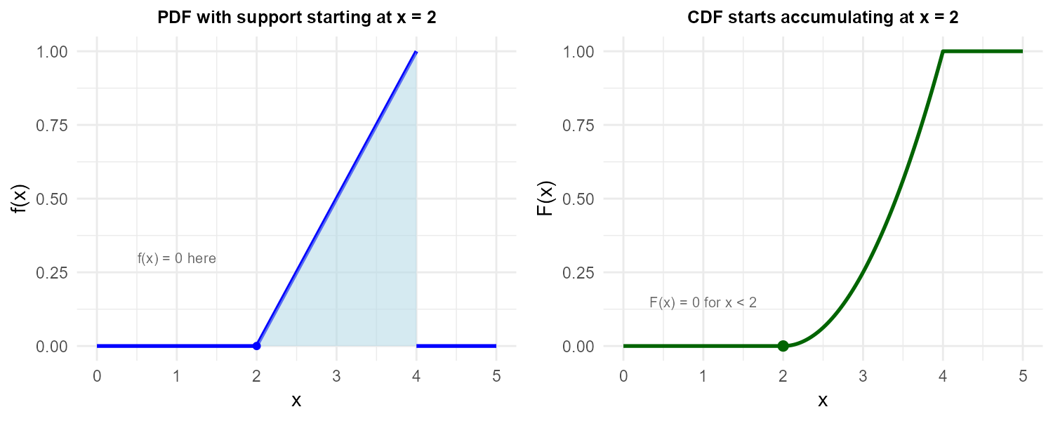
Fig. 6.18 The CDF starts accumulating at \(x = 2\), not \(x = 0\).

Part (c): P(X ≤ 3)

\[P(X \leq 3) = F_X(3) = \frac{(3-2)^2}{4} = \frac{1}{4} = 0.25\]

Part (d): P(2.5 < X < 3.5)

\[P(2.5 < X < 3.5) = F_X(3.5) - F_X(2.5) = \frac{(1.5)^2}{4} - \frac{(0.5)^2}{4} = \frac{2.25 - 0.25}{4} = \frac{2}{4} = 0.5\]

Part (e): 75th percentile

Solve \(F_X(x_{0.75}) = 0.75\):

\[\frac{(x_{0.75} - 2)^2}{4} = 0.75\]

\[(x_{0.75} - 2)^2 = 3\]

\[x_{0.75} = 2 + \sqrt{3} \approx 3.732 \text{ mg/L}\]

Part (f): Common Mistake

The student integrated from 0, but the PDF equals 0 for \(x < 2\). The CDF is defined as:

\[F_X(x) = \int_{-\infty}^{x} f_X(t) \, dt\]

Since \(f_X(t) = 0\) for \(t < 2\), the integral from \(-\infty\) to 2 contributes nothing. The correct calculation integrates only over the support where \(f_X > 0\).

---

Exercise 3: Piecewise CDF Construction

A computer scientist models network latency \(X\) (in milliseconds) with PDF:

\[\begin{split}f_X(x) = \begin{cases} \frac{x}{3}, & 0 \leq x \leq 2\\ \frac{1}{3}, & 2 < x \leq 3\\ 0, & \text{elsewhere} \end{cases}\end{split}\]

1. Verify this is a valid PDF.

2. Construct the complete piecewise CDF.

3. Use the CDF to find \(P(1 < X \leq 2.5)\).

4. Find the median latency.

5. Find the 90th percentile.

6. Find the interquartile range (IQR).

Solution

Part (a): Verify PDF validity

Non-negativity: Both pieces are non-negative on their domains. ✓

Total area = 1:

\[\int_{0}^{2} \frac{x}{3} \, dx + \int_{2}^{3} \frac{1}{3} \, dx = \frac{1}{3} \cdot \frac{x^2}{2}\Bigg|_0^2 + \frac{1}{3} \cdot 1 = \frac{1}{3} \cdot 2 + \frac{1}{3} = \frac{2}{3} + \frac{1}{3} = 1 \text{ ✓}\]

Part (b): Construct piecewise CDF

Region 1 (\(x < 0\)):

\[F_X(x) = 0\]

Region 2 (\(0 \leq x \leq 2\)):

\[F_X(x) = \int_{0}^{x} \frac{t}{3} \, dt = \frac{x^2}{6}\]

Check: \(F_X(2) = \frac{4}{6} = \frac{2}{3}\)

Region 3 (\(2 < x \leq 3\)):

\[F_X(x) = F_X(2) + \int_{2}^{x} \frac{1}{3} \, dt = \frac{2}{3} + \frac{x-2}{3} = \frac{x}{3}\]

Check: \(F_X(3) = 1\) ✓

Region 4 (\(x > 3\)):

\[F_X(x) = 1\]

Complete CDF:

\[\begin{split}F_X(x) = \begin{cases} 0, & x < 0\\ \frac{x^2}{6}, & 0 \leq x \leq 2\\ \frac{x}{3}, & 2 < x \leq 3\\ 1, & x > 3 \end{cases}\end{split}\]

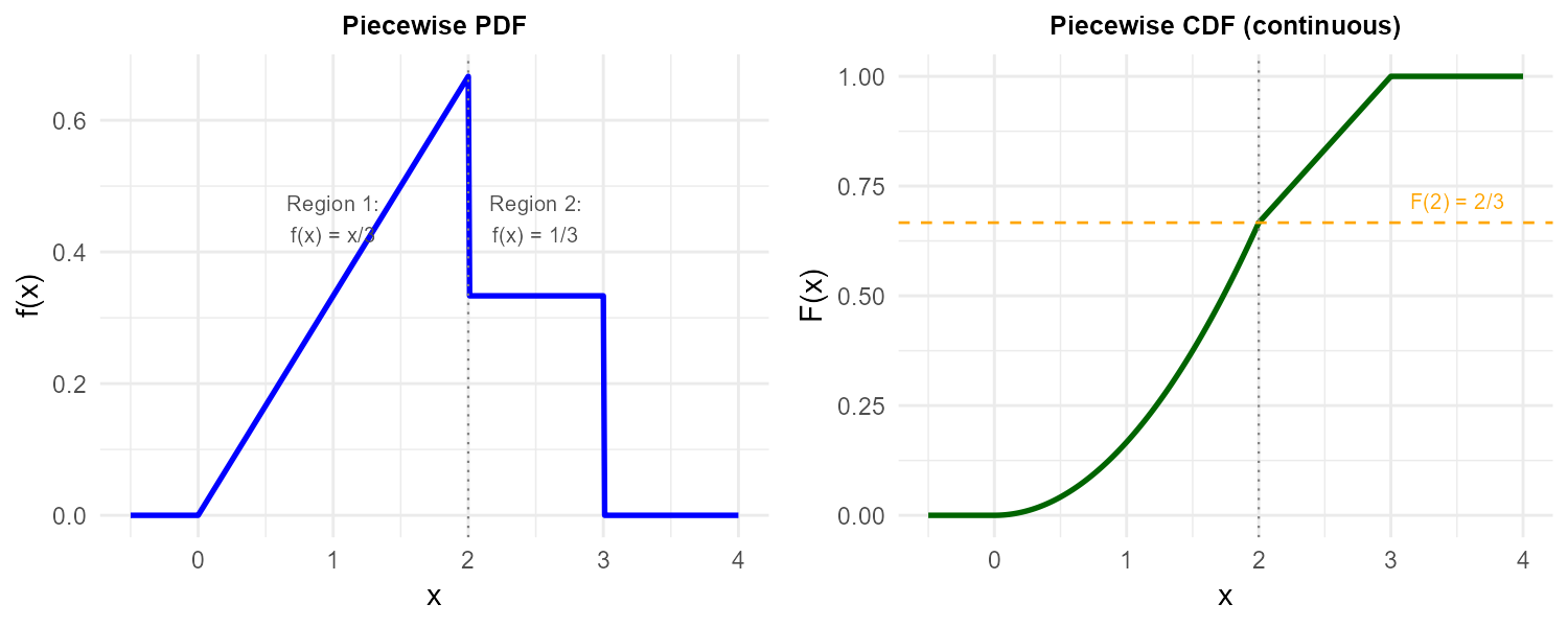
Fig. 6.19 Piecewise PDF (left) and its CDF (right). Note the CDF is continuous but has different formulas in each region.

Part (c): P(1 < X ≤ 2.5)

\[P(1 < X \leq 2.5) = F_X(2.5) - F_X(1) = \frac{2.5}{3} - \frac{1}{6} = \frac{5}{6} - \frac{1}{6} = \frac{4}{6} = \frac{2}{3}\]

Part (d): Median

We need \(F_X(x_{0.5}) = 0.5\).

Since \(F_X(2) = \frac{2}{3} > 0.5\), the median is in Region 2.

\[\frac{x_{0.5}^2}{6} = 0.5 \implies x_{0.5}^2 = 3 \implies x_{0.5} = \sqrt{3} \approx 1.732 \text{ ms}\]

Part (e): 90th percentile

Since \(F_X(2) = \frac{2}{3} \approx 0.667 < 0.9\), the 90th percentile is in Region 3.

\[\frac{x_{0.9}}{3} = 0.9 \implies x_{0.9} = 2.7 \text{ ms}\]

Part (f): IQR

25th percentile: \(F_X(2) = 0.667 > 0.25\), so use Region 2:

\[\frac{x_{0.25}^2}{6} = 0.25 \implies x_{0.25}^2 = 1.5 \implies x_{0.25} = \sqrt{1.5} \approx 1.225 \text{ ms}\]

75th percentile: \(F_X(2) = 0.667 < 0.75\), so use Region 3:

\[\frac{x_{0.75}}{3} = 0.75 \implies x_{0.75} = 2.25 \text{ ms}\]

IQR:

\[\text{IQR} = x_{0.75} - x_{0.25} = 2.25 - 1.225 = 1.025 \text{ ms}\]

---

Exercise 4: Piecewise CDF with Gap in Support

An industrial engineer models machine cycle time \(X\) (in seconds) with PDF:

\[\begin{split}f_X(x) = \begin{cases} \frac{1}{3}, & 0 \leq x \leq 2\\ \frac{1}{6}(x - 4), & 4 \leq x \leq 6\\ 0, & \text{elsewhere} \end{cases}\end{split}\]

Note the gap in support from \(x = 2\) to \(x = 4\).

1. Verify this is a valid PDF.

2. Construct the complete piecewise CDF, including the gap region.

3. Find \(P(1 < X < 5)\).

4. Find the median.

5. If a cycle takes more than 4 seconds (slow mode), what is \(P(X > 5 | X > 4)\)?

Solution

Part (a): Verify PDF validity

Non-negativity: Region 1 has constant positive density. Region 2 has \(x - 4 \geq 0\) for \(x \geq 4\). ✓

Total area = 1:

\[\int_{0}^{2} \frac{1}{3} \, dx + \int_{4}^{6} \frac{1}{6}(x - 4) \, dx = \frac{2}{3} + \frac{1}{6} \cdot \frac{(x-4)^2}{2}\Bigg|_4^6\]

\[= \frac{2}{3} + \frac{1}{12} \cdot 4 = \frac{2}{3} + \frac{1}{3} = 1 \text{ ✓}\]

Part (b): Construct piecewise CDF

Region 1 (\(x < 0\)): \(F_X(x) = 0\)

Region 2 (\(0 \leq x \leq 2\)):

\[F_X(x) = \int_0^x \frac{1}{3} \, dt = \frac{x}{3}\]

\(F_X(2) = \frac{2}{3}\)

Region 3 (\(2 < x < 4\)): Gap region — no new probability accumulates

\[F_X(x) = F_X(2) = \frac{2}{3}\]

Note: \(F_X(4) = \frac{2}{3}\) as well (the CDF remains constant through the gap).

Region 4 (\(4 \leq x \leq 6\)):

\[F_X(x) = F_X(4) + \int_4^x \frac{1}{6}(t-4) \, dt = \frac{2}{3} + \frac{(x-4)^2}{12}\]

\(F_X(6) = \frac{2}{3} + \frac{4}{12} = \frac{2}{3} + \frac{1}{3} = 1\) ✓

Region 5 (\(x > 6\)): \(F_X(x) = 1\)

Complete CDF:

\[\begin{split}F_X(x) = \begin{cases} 0, & x < 0\\ \frac{x}{3}, & 0 \leq x \leq 2\\ \frac{2}{3}, & 2 < x < 4\\ \frac{2}{3} + \frac{(x-4)^2}{12}, & 4 \leq x \leq 6\\ 1, & x > 6 \end{cases}\end{split}\]

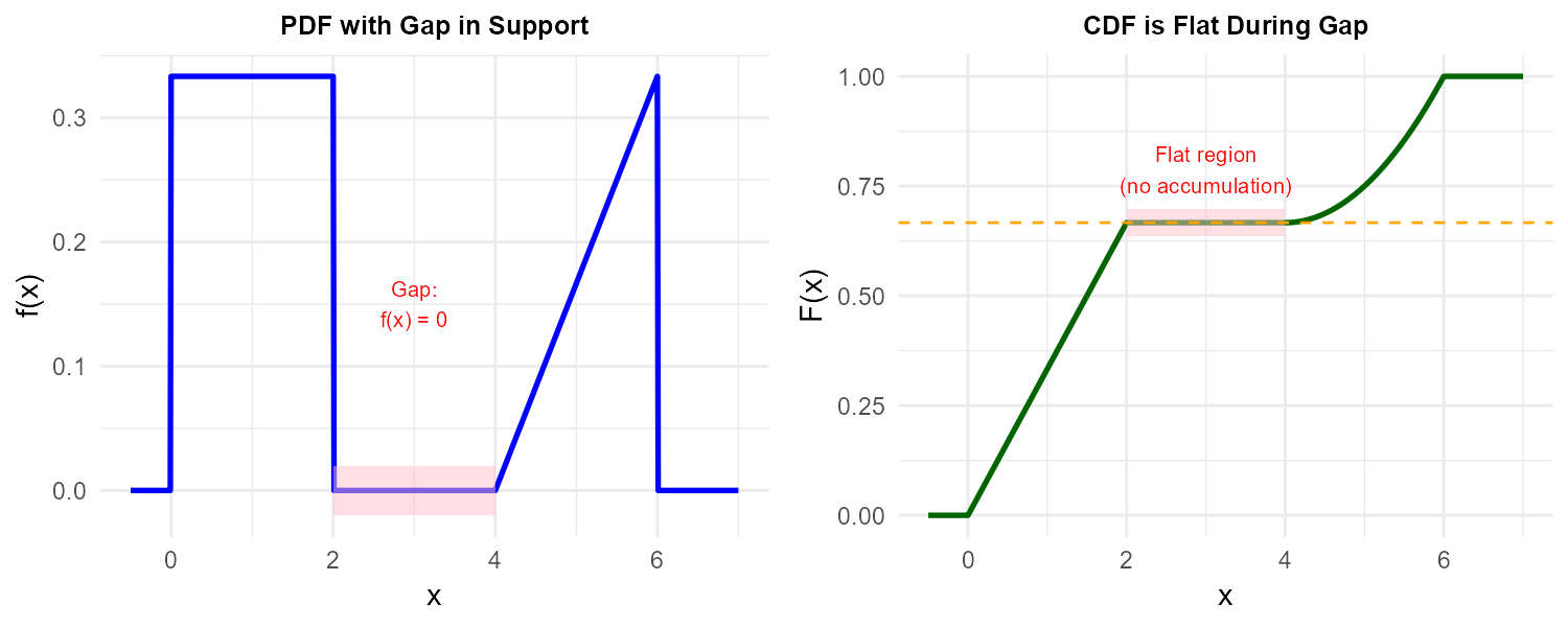
Fig. 6.20 The CDF is flat (horizontal) during the gap where the PDF is zero.

Part (c): P(1 < X < 5)

\[P(1 < X < 5) = F_X(5) - F_X(1) = \left[\frac{2}{3} + \frac{1}{12}\right] - \frac{1}{3} = \frac{3}{4} - \frac{1}{3} = \frac{9-4}{12} = \frac{5}{12}\]

Part (d): Median

Since \(F_X(2) = \frac{2}{3} > 0.5\), the median is in Region 2.

\[\frac{x_{0.5}}{3} = 0.5 \implies x_{0.5} = 1.5 \text{ seconds}\]

Part (e): Conditional probability

\[P(X > 5 | X > 4) = \frac{P(X > 5)}{P(X > 4)} = \frac{1 - F_X(5)}{1 - F_X(4)}\]

\[= \frac{1 - \frac{3}{4}}{1 - \frac{2}{3}} = \frac{1/4}{1/3} = \frac{3}{4}\]

---

Exercise 5: From CDF to PDF (Differentiation)

A materials engineer is given the following CDF for material strength \(X\) (in MPa):

\[\begin{split}F_X(x) = \begin{cases} 0, & x < 0\\ \frac{x^3}{8}, & 0 \leq x \leq 2\\ 1, & x > 2 \end{cases}\end{split}\]

1. Find the PDF \(f_X(x)\) by differentiating the CDF.

2. Verify your PDF integrates to 1.

3. Find \(P(X > 1.5)\).

4. Find the median strength.

5. Find the 25th and 75th percentiles, then compute the IQR.

Solution

Part (a): Find PDF by differentiation

The PDF is the derivative of the CDF: \(f_X(x) = \frac{d}{dx}F_X(x)\).

Region \(0 \leq x \leq 2\):

\[f_X(x) = \frac{d}{dx}\left(\frac{x^3}{8}\right) = \frac{3x^2}{8}\]

Complete PDF:

\[\begin{split}f_X(x) = \begin{cases} \frac{3x^2}{8}, & 0 \leq x \leq 2\\ 0, & \text{elsewhere} \end{cases}\end{split}\]

Part (b): Verify PDF integrates to 1

\[\int_0^2 \frac{3x^2}{8} \, dx = \frac{3}{8} \cdot \frac{x^3}{3}\Bigg|_0^2 = \frac{1}{8} \cdot 8 = 1 \text{ ✓}\]

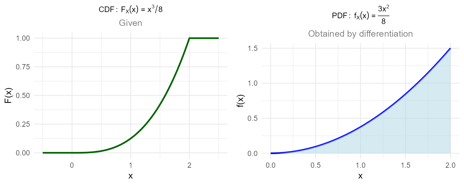
Fig. 6.21 The PDF is the derivative of the CDF. Where the CDF rises steeply, the PDF is large.

Part (c): P(X > 1.5)

\[P(X > 1.5) = 1 - F_X(1.5) = 1 - \frac{(1.5)^3}{8} = 1 - \frac{3.375}{8} = 1 - 0.422 = 0.578\]

Part (d): Median

Solve \(F_X(x_{0.5}) = 0.5\):

\[\frac{x_{0.5}^3}{8} = 0.5 \implies x_{0.5}^3 = 4 \implies x_{0.5} = \sqrt[3]{4} \approx 1.587 \text{ MPa}\]

Part (e): Quartiles and IQR

25th percentile:

\[\frac{x_{0.25}^3}{8} = 0.25 \implies x_{0.25}^3 = 2 \implies x_{0.25} = \sqrt[3]{2} \approx 1.260 \text{ MPa}\]

75th percentile:

\[\frac{x_{0.75}^3}{8} = 0.75 \implies x_{0.75}^3 = 6 \implies x_{0.75} = \sqrt[3]{6} \approx 1.817 \text{ MPa}\]

IQR:

\[\text{IQR} = x_{0.75} - x_{0.25} = \sqrt[3]{6} - \sqrt[3]{2} \approx 1.817 - 1.260 = 0.557 \text{ MPa}\]

---

Exercise 6: Exponential CDF

A reliability engineer models time-to-failure \(X\) (in hours) for an electronic component with CDF:

\[\begin{split}F_X(x) = \begin{cases} 0, & x < 0\\ 1 - e^{-x/100}, & x \geq 0 \end{cases}\end{split}\]

1. Find the PDF by differentiation.

2. Find \(P(X > 150)\), the probability a component lasts more than 150 hours.

3. Find the median lifetime.

4. Find the 95th percentile (often used as a “design life” specification).

5. If a component has already survived 50 hours, find \(P(X > 150 | X > 50)\).

Solution

Part (a): Find PDF

\[f_X(x) = \frac{d}{dx}\left(1 - e^{-x/100}\right) = \frac{1}{100}e^{-x/100} \text{ for } x \geq 0\]

This is an exponential distribution with rate \(\lambda = \frac{1}{100}\) (or mean \(\mu = 100\) hours).

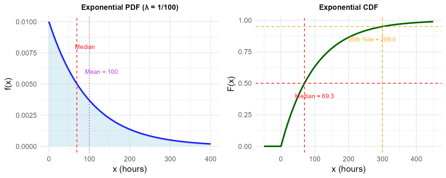
Fig. 6.22 Exponential distribution: PDF decays exponentially; CDF approaches 1 asymptotically.

Part (b): P(X > 150)

\[P(X > 150) = 1 - F_X(150) = 1 - (1 - e^{-150/100}) = e^{-1.5} \approx 0.223\]

Part (c): Median

Solve \(F_X(x_{0.5}) = 0.5\):

\[1 - e^{-x_{0.5}/100} = 0.5 \implies e^{-x_{0.5}/100} = 0.5\]

\[-\frac{x_{0.5}}{100} = \ln(0.5) = -\ln(2) \implies x_{0.5} = 100\ln(2) \approx 69.3 \text{ hours}\]

Part (d): 95th percentile

Solve \(F_X(x_{0.95}) = 0.95\):

\[1 - e^{-x_{0.95}/100} = 0.95 \implies e^{-x_{0.95}/100} = 0.05\]

\[-\frac{x_{0.95}}{100} = \ln(0.05) \implies x_{0.95} = -100\ln(0.05) = 100\ln(20) \approx 299.6 \text{ hours}\]

Part (e): Memoryless property

For exponential distributions:

\[P(X > 150 | X > 50) = P(X > 100) = e^{-100/100} = e^{-1} \approx 0.368\]

The probability of surviving an additional 100 hours is the same regardless of how long the component has already lasted. This is the memoryless property unique to exponential distributions.

---

Exercise 7: Verifying CDF Validity

Determine whether each of the following could be a valid CDF. If valid, find the corresponding PDF. If not valid, explain which property is violated.

1. \(F(x) = \begin{cases} 0, & x < 0\\ x^2, & 0 \leq x \leq 1\\ 1, & x > 1 \end{cases}\)

2. \(F(x) = \begin{cases} 0, & x < 0\\ 2x - x^2, & 0 \leq x \leq 1\\ 1, & x > 1 \end{cases}\)

3. \(F(x) = \begin{cases} 0, & x < 1\\ \frac{x-1}{2}, & 1 \leq x \leq 3\\ 1, & x > 3 \end{cases}\)

4. \(F(x) = \begin{cases} 0, & x < 0\\ x^3 - x^2, & 0 \leq x \leq 1\\ 1, & x > 1 \end{cases}\)

Solution

Part (a): Valid CDF

Check properties:

• Monotonicity: \(F'(x) = 2x \geq 0\) for \(x \in [0,1]\). ✓

• Limits: \(F(-\infty) = 0\), \(F(\infty) = 1\). ✓

• Right-continuous: Continuous everywhere. ✓

• Boundary values: \(F(0) = 0\), \(F(1) = 1\). ✓

PDF: \(f(x) = 2x\) for \(0 \leq x \leq 1\), 0 elsewhere.

Part (b): Valid CDF

Check properties:

• Monotonicity: \(F'(x) = 2 - 2x = 2(1-x) \geq 0\) for \(x \in [0,1]\). ✓

• Limits: \(F(-\infty) = 0\), \(F(\infty) = 1\). ✓

• Boundary values: \(F(0) = 0\), \(F(1) = 2 - 1 = 1\). ✓

PDF: \(f(x) = 2 - 2x = 2(1-x)\) for \(0 \leq x \leq 1\), 0 elsewhere.

Part (c): Valid CDF

Check properties:

• Monotonicity: \(F'(x) = \frac{1}{2} > 0\). ✓

• Limits: ✓

• Boundary values: \(F(1) = 0\), \(F(3) = 1\). ✓

PDF: \(f(x) = \frac{1}{2}\) for \(1 \leq x \leq 3\), 0 elsewhere. (Uniform distribution on [1, 3])

Part (d): NOT a valid CDF

Check monotonicity: \(F'(x) = 3x^2 - 2x = x(3x - 2)\).

For \(0 < x < \frac{2}{3}\), we have \(3x - 2 < 0\), so \(F'(x) < 0\).

Violations:

1. Negative values: On \((0, 1)\), \(F(x) = x^3 - x^2 = x^2(x-1) \leq 0\) since \(x - 1 < 0\). A CDF must satisfy \(0 \leq F(x) \leq 1\) for all \(x\).

2. Not nondecreasing: The derivative is negative on \((0, \frac{2}{3})\), so the function decreases on part of \([0,1]\).

3. Right-continuity failure at \(x = 1\): With the piecewise definition, \(F(1) = 1^3 - 1^2 = 0\) from the middle piece, but \(\lim_{x \to 1^+} F(x) = 1\) from the right piece. Since \(F(1) \neq \lim_{x \to 1^+} F(x)\), right-continuity fails.

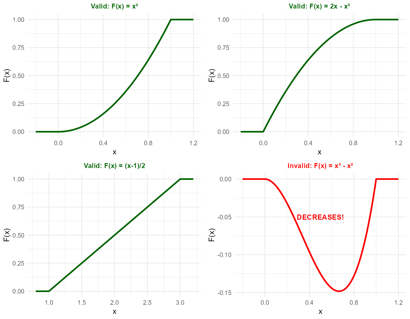
Fig. 6.23 Top row: Valid CDFs are non-decreasing. Bottom: Invalid CDF decreases in the middle.

---

Exercise 8: Symmetric Distribution Percentiles

A sensor measurement error \(X\) (in μV) has the symmetric triangular PDF:

\[\begin{split}f_X(x) = \begin{cases} \frac{1}{4}(x + 2), & -2 \leq x \leq 0\\ \frac{1}{4}(2 - x), & 0 < x \leq 2\\ 0, & \text{elsewhere} \end{cases}\end{split}\]

1. Verify this is a valid PDF.

2. Use symmetry to determine the median without calculation.

3. Construct the CDF.

4. Find the 10th and 90th percentiles.

5. Verify that \(x_{0.1}\) and \(x_{0.9}\) are symmetric about the median.

Solution

Part (a): Verify PDF

The PDF forms a triangle with base 4 (from -2 to 2) and height \(\frac{1}{2}\) (at x = 0).

Area = \(\frac{1}{2} \times 4 \times \frac{1}{2} = 1\) ✓

Part (b): Median by symmetry

The PDF is symmetric about \(x = 0\). By symmetry, the median is:

\[x_{0.5} = 0 \text{ μV}\]

Part (c): Construct CDF

Region 1 (\(x < -2\)): \(F_X(x) = 0\)

Region 2 (\(-2 \leq x \leq 0\)):

\[F_X(x) = \int_{-2}^{x} \frac{1}{4}(t + 2) \, dt = \frac{1}{4} \cdot \frac{(t+2)^2}{2}\Bigg|_{-2}^x = \frac{(x+2)^2}{8}\]

\(F_X(0) = \frac{4}{8} = \frac{1}{2}\) ✓ (confirms median at 0)

Region 3 (\(0 < x \leq 2\)):

\[F_X(x) = \frac{1}{2} + \int_{0}^{x} \frac{1}{4}(2 - t) \, dt = \frac{1}{2} + \frac{1}{4}\left[2t - \frac{t^2}{2}\right]_0^x = \frac{1}{2} + \frac{x}{2} - \frac{x^2}{8}\]

Or equivalently: \(F_X(x) = 1 - \frac{(2-x)^2}{8}\) (by symmetry)

Region 4 (\(x > 2\)): \(F_X(x) = 1\)

Complete CDF:

\[\begin{split}F_X(x) = \begin{cases} 0, & x < -2\\ \frac{(x+2)^2}{8}, & -2 \leq x \leq 0\\ 1 - \frac{(2-x)^2}{8}, & 0 < x \leq 2\\ 1, & x > 2 \end{cases}\end{split}\]

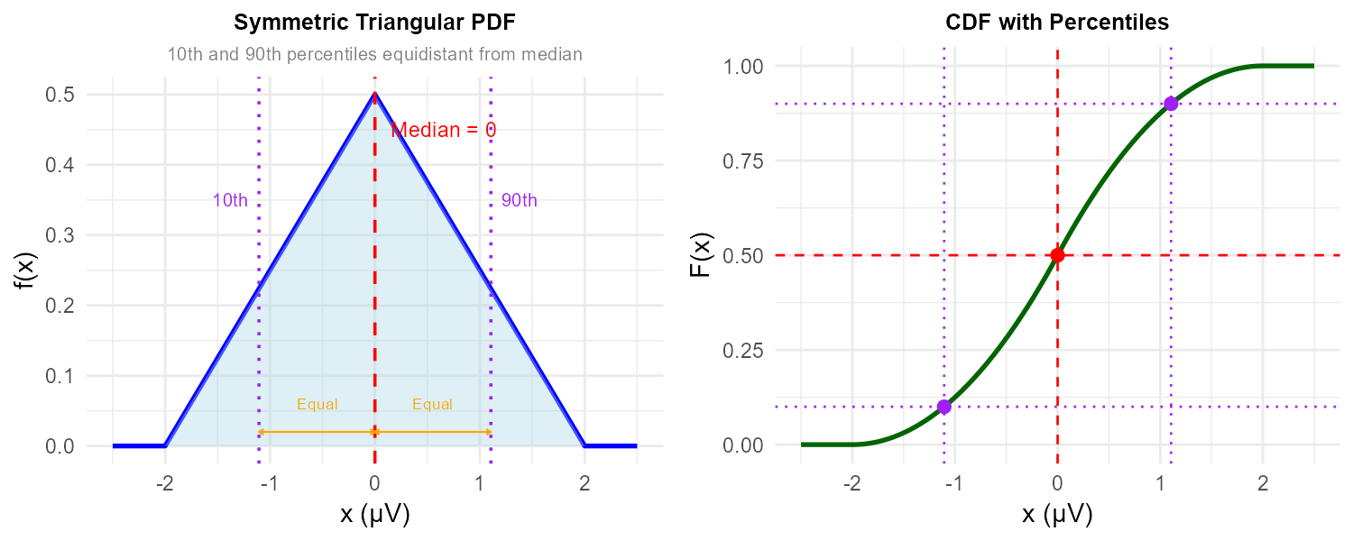
Fig. 6.24 Symmetric triangular PDF with 10th and 90th percentiles marked equidistant from the median.

Part (d): 10th and 90th percentiles

10th percentile (in Region 2 since \(0.1 < 0.5\)):

\[\frac{(x_{0.1} + 2)^2}{8} = 0.1 \implies (x_{0.1} + 2)^2 = 0.8\]

\[x_{0.1} = -2 + \sqrt{0.8} = -2 + 0.894 \approx -1.106 \text{ μV}\]

90th percentile (by symmetry, or using Region 3):

\[1 - \frac{(2 - x_{0.9})^2}{8} = 0.9 \implies (2 - x_{0.9})^2 = 0.8\]

\[x_{0.9} = 2 - \sqrt{0.8} \approx 1.106 \text{ μV}\]

Part (e): Verify symmetry

We show \(x_{0.1} = -x_{0.9}\):

\[x_{0.1} = -2 + \sqrt{0.8} = -(2 - \sqrt{0.8}) = -x_{0.9}\]

Therefore the distances from the median (0) are equal:

\[|x_{0.1} - 0| = |x_{0.9} - 0| = 2 - \sqrt{0.8} \approx 1.106 \text{ ✓}\]

---

Exercise 9: Working Backwards from Percentiles

A manufacturing process produces components whose length \(X\) (in cm) follows a distribution with CDF:

\[\begin{split}F_X(x) = \begin{cases} 0, & x < a\\ \left(\frac{x - a}{b - a}\right)^2, & a \leq x \leq b\\ 1, & x > b \end{cases}\end{split}\]

The quality control team has determined that:

• The 25th percentile is 12 cm

• The 75th percentile is 16 cm

1. Set up a system of equations using these percentile conditions.

2. Solve for the parameters \(a\) and \(b\).

3. Find the median length.

4. Find the PDF.

Solution

Part (a): System of equations

Using \(F_X(x_{0.25}) = 0.25\) and \(F_X(x_{0.75}) = 0.75\):

\[\left(\frac{12 - a}{b - a}\right)^2 = 0.25 \implies \frac{12 - a}{b - a} = 0.5\]

\[\left(\frac{16 - a}{b - a}\right)^2 = 0.75 \implies \frac{16 - a}{b - a} = \sqrt{0.75} = \frac{\sqrt{3}}{2}\]

Part (b): Solve for a and b

From equation 1: \(12 - a = 0.5(b - a)\), so \(24 - 2a = b - a\), giving \(b = 24 - a\).

Substitute into equation 2:

\[\frac{16 - a}{24 - 2a} = \frac{\sqrt{3}}{2}\]

\[2(16 - a) = \sqrt{3}(24 - 2a)\]

\[32 - 2a = 24\sqrt{3} - 2\sqrt{3}a\]

\[32 - 24\sqrt{3} = 2a - 2\sqrt{3}a = 2a(1 - \sqrt{3})\]

\[a = \frac{32 - 24\sqrt{3}}{2(1 - \sqrt{3})} = \frac{16 - 12\sqrt{3}}{1 - \sqrt{3}}\]

Rationalizing: multiply by \(\frac{1 + \sqrt{3}}{1 + \sqrt{3}}\):

\[a = \frac{(16 - 12\sqrt{3})(1 + \sqrt{3})}{(1 - \sqrt{3})(1 + \sqrt{3})} = \frac{16 + 16\sqrt{3} - 12\sqrt{3} - 36}{1 - 3}\]

\[= \frac{-20 + 4\sqrt{3}}{-2} = 10 - 2\sqrt{3} \approx 6.54 \text{ cm}\]

Then: \(b = 24 - a = 24 - 10 + 2\sqrt{3} = 14 + 2\sqrt{3} \approx 17.46 \text{ cm}\)

Part (c): Median

\[\left(\frac{x_{0.5} - a}{b - a}\right)^2 = 0.5 \implies \frac{x_{0.5} - a}{b - a} = \frac{1}{\sqrt{2}}\]

\[x_{0.5} = a + \frac{b - a}{\sqrt{2}} = (10 - 2\sqrt{3}) + \frac{4 + 4\sqrt{3}}{\sqrt{2}}\]

\[= 10 - 2\sqrt{3} + 2\sqrt{2} + 2\sqrt{6} \approx 14.23 \text{ cm}\]

Part (d): PDF

\[f_X(x) = \frac{d}{dx}\left[\left(\frac{x - a}{b - a}\right)^2\right] = \frac{2(x - a)}{(b - a)^2}\]

With \(b - a = 4 + 4\sqrt{3}\):

\[f_X(x) = \frac{2(x - a)}{(4 + 4\sqrt{3})^2} = \frac{x - a}{8(1 + \sqrt{3})^2} \text{ for } a \leq x \leq b\]

---

6.3.10. Additional Practice Problems

True/False Questions (1 point each)

1. For a continuous random variable, \(F_X(a) = P(X < a)\) and \(F_X(a) = P(X \leq a)\) give the same value.

   Ⓣ or Ⓕ

2. A valid CDF must satisfy \(F_X(x) \leq 1\) for all \(x\).

   Ⓣ or Ⓕ

3. If \(F_X(5) = 0.7\), then \(P(X > 5) = 0.3\).

   Ⓣ or Ⓕ

4. The PDF can be obtained from the CDF by integration.

   Ⓣ or Ⓕ

5. In a region where the PDF equals zero, the CDF must also equal zero.

   Ⓣ or Ⓕ

6. The median of a continuous random variable is the value \(x\) where \(F_X(x) = 0.5\).

   Ⓣ or Ⓕ

7. For any valid CDF, \(F_X(b) - F_X(a) \geq 0\) when \(b > a\).

   Ⓣ or Ⓕ

8. If \(X\) has a symmetric PDF about \(c\), then the median equals \(c\).

   Ⓣ or Ⓕ

Multiple Choice Questions (2 points each)

9. If \(F_X(x) = x^3\) for \(0 \leq x \leq 1\), what is \(P(0.5 < X < 0.8)\)?

   Ⓐ 0.300

   Ⓑ 0.387

   Ⓒ 0.512

   Ⓓ 0.637

10. If \(F_X(x) = 1 - e^{-2x}\) for \(x \geq 0\), what is the PDF?

    Ⓐ \(f_X(x) = e^{-2x}\)

    Ⓑ \(f_X(x) = 2e^{-2x}\)

    Ⓒ \(f_X(x) = -2e^{-2x}\)

    Ⓓ \(f_X(x) = 1 - e^{-2x}\)

11. For a CDF with \(F_X(3) = 0.4\) and \(F_X(7) = 0.9\), what is \(P(3 < X \leq 7)\)?

    Ⓐ 0.36

    Ⓑ 0.50

    Ⓒ 0.54

    Ⓓ 0.90

12. If \(F_X(x) = \frac{x^2}{16}\) for \(0 \leq x \leq 4\), what is the median?

    Ⓐ 2

    Ⓑ \(2\sqrt{2}\)

    Ⓒ \(\sqrt{8}\)

    Ⓓ Both Ⓑ and Ⓒ

13. Which function could NOT be a valid CDF?

    Ⓐ \(F(x) = \frac{1}{1 + e^{-x}}\) for all \(x\)

    Ⓑ \(F(x) = \sin(x)\) for \(0 \leq x \leq \frac{\pi}{2}\), 0 for \(x < 0\), 1 for \(x > \frac{\pi}{2}\)

    Ⓒ \(F(x) = x - x^2\) for \(0 \leq x \leq 1\), 0 for \(x < 0\), 1 for \(x > 1\)

    Ⓓ \(F(x) = 1 - \frac{1}{x}\) for \(x \geq 1\), 0 for \(x < 1\)

14. For \(F_X(x) = \frac{(x-2)^2}{9}\) on \(2 \leq x \leq 5\), what is the 75th percentile?

    Ⓐ 3.50

    Ⓑ 4.25

    Ⓒ 4.60

    Ⓓ 4.75

Answers to Practice Problems

True/False Answers:

1. True — For continuous random variables, \(P(X = a) = 0\), so \(P(X < a) = P(X \leq a)\).

2. True — By definition, \(F_X(x) = P(X \leq x)\), and all probabilities are at most 1.

3. True — \(P(X > 5) = 1 - P(X \leq 5) = 1 - F_X(5) = 1 - 0.7 = 0.3\).

4. False — The PDF is obtained by differentiation: \(f_X(x) = F_X'(x)\). The CDF is obtained from the PDF by integration.

5. False — The CDF is flat (constant) where the PDF is zero, but it retains the accumulated probability from previous regions. It only equals zero before the start of support.

6. True — By definition, the \(p\)-th percentile is \(x_p\) where \(F_X(x_p) = p\). The median is the 50th percentile.

7. True — CDFs are non-decreasing, so \(b > a\) implies \(F_X(b) \geq F_X(a)\).

8. True — For symmetric distributions, the median equals the center of symmetry.

Multiple Choice Answers:

9. Ⓑ — \(P(0.5 < X < 0.8) = F_X(0.8) - F_X(0.5) = 0.8^3 - 0.5^3 = 0.512 - 0.125 = 0.387\).

10. Ⓑ — \(f_X(x) = \frac{d}{dx}(1 - e^{-2x}) = 2e^{-2x}\).

11. Ⓑ — \(P(3 < X \leq 7) = F_X(7) - F_X(3) = 0.9 - 0.4 = 0.5\).

12. Ⓓ — Solve \(\frac{x^2}{16} = 0.5\), giving \(x^2 = 8\), so \(x = \sqrt{8} = 2\sqrt{2}\). Both Ⓑ and Ⓒ are correct (they’re the same number).

13. Ⓒ — For \(F(x) = x - x^2\), the derivative is \(F'(x) = 1 - 2x\), which is negative for \(x > 0.5\). This means the function decreases on \((0.5, 1)\), violating the monotonicity requirement.

14. Ⓒ — Solve \(\frac{(x-2)^2}{9} = 0.75\), giving \((x-2)^2 = 6.75\), so \(x = 2 + \sqrt{6.75} \approx 4.60\).