Slides 📊

Download Chapter 13 slides (PPTX)

13.2. Simple Linear Regression

After identifying a linear association between two quantitative variables via a scatter plot, we proceed to mathematical modeling of the association. This involves formalizing the population model, developing methods to estimate the model parameters, and assessing the model’s fit to the data.

Road Map 🧭

• Understand the implications of linear regression model assumptions.

• Derive the least squares estimates of the slope and intercept parameters, and present the result as a fitted regression line.

• Use the ANOVA table to decompose the sources of variability in the repsonse into error and model components.

• Use the coefficient of determination and the sample correlation as assisting numerical summaries.

13.2.1. The Simple Linear Regression Model

In this course, we assume that the \(X\) values are given (non-random) as \(x_1, x_2, \cdots, x_n\). For each explanatory value, the corresponding response \(Y_i\) is generated from the population model:

(13.1)\[Y_i = \beta_0 + \beta_1 x_i + \varepsilon_i,\]

where \(\varepsilon_i \stackrel{iid}{\sim} N(0, \sigma^2)\), and \(\beta_0\) and \(\beta_1\) are the intercept and slope of the true linear association.

Important Implications of the Model

1. The Mean Response

\(y=\beta_0 + \beta_1 x\) represents the mean response line, or the true relationship between the explanatory and response variables. That is,

\[\begin{split}E[Y|X=x] &= E[\beta_0 + \beta_1 x + \varepsilon] \\ &= \beta_0 + \beta_1 x + E[\varepsilon]\\ &= \beta_0 + \beta_1 x,\end{split}\]

for any given \(x\) values in an appropriate range. \(\beta_0\), \(\beta_1\), and \(x\) pass through the expectation operator unchanged since they are constants. The error term has expected value zero, so it disappears.

2. The Error Term

The error term \(\varepsilon\) represents the random variation in \(Y\) that is not explained by the mean response line. With non-random explanatory values, this is the only source of randomness in \(Y\). Namely,

\[\text{Var}(Y|X=x) = \text{Var}(\beta_0 + \beta_1 x + \varepsilon) = \text{Var}(\varepsilon) = \sigma^2.\]

Note that the result does not depend on the index \(i\) or the value of \(x_i\). In our model, we assume that the true spread of \(Y\) values around the regression line remains constant regardless of the \(X\) value.

3. The Conditional distribution of \(Y_i\)

With the explanatory value fixed as \(x_i\), each \(Y_i\) is a linear function of a normal random variable \(\varepsilon_i\). This implies that \(Y_i|X=x_i\) is also normally distributed. Combining this result with the previous two observations, we can write the exact conditional distribution of the response as:

\[Y_i|X=x_i \sim N(\beta_0 + \beta_1 x_i, \quad \sigma^2)\]

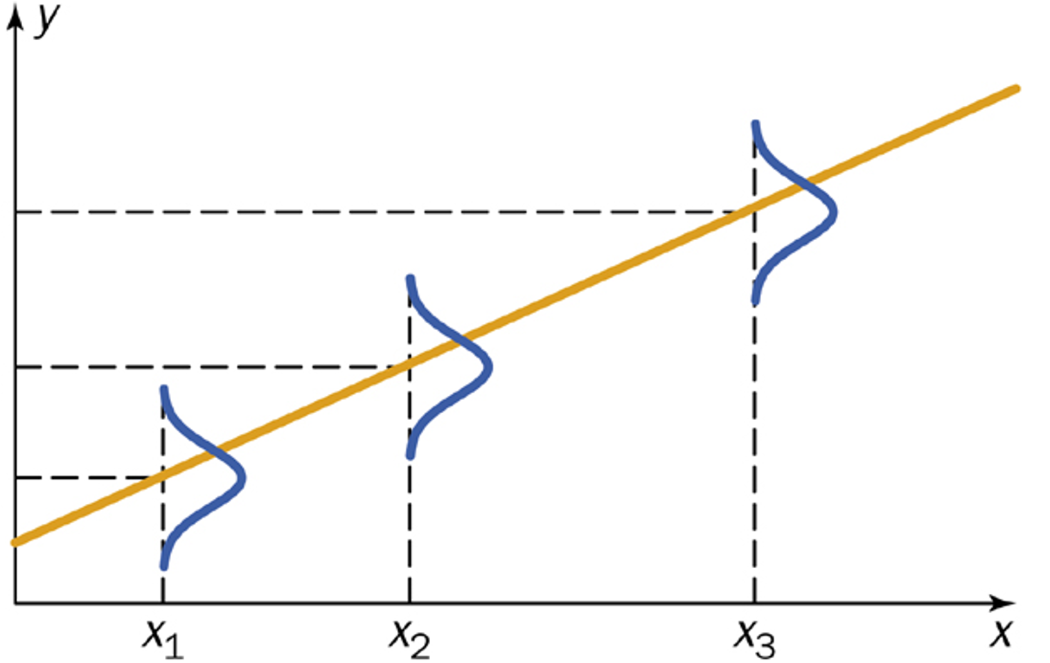
Fig. 13.13 Visualization of conditional distributions of \(Y_i\) given \(x_i\)

Summary of the Essential Assumptions

The following four assumptions are equivalent to the model assumptions discussed above and are required to ensure validity of subsequent analysis procedures.

• Assumption 1: Independence

  For each given value \(x_i\), \(Y_i\) is a size-1 simple random sample from the distribution of \(Y|X=x_i\). Further, the pairs \((x_i, Y_i)\) are independent from all other pairs \((x_j, Y_j)\), \(j\neq i\).

• Assumption 2: Linearity

  The association between the explanatory variable and the response is linear on average.

• Assumption 3: Normality

  The errors are normally distributed:

  \[\varepsilon_i \stackrel{iid}{\sim} N(0, \sigma^2) \quad \text{for } i = 1, 2, \ldots, n\]

• Assumption 4: Equal Variance

  The error terms have constant variance \(\sigma^2\) across all values of \(X\).

13.2.2. Point Estimates of Slope and Intercept

We now develop the point estimates for the unknown intercept and slope parameters \(\beta_0\) and \(\beta_1\) using the least squares method. The estimators are chosen so that the resulting trend line yields the smallest possible overall squared distance from the observed response values.

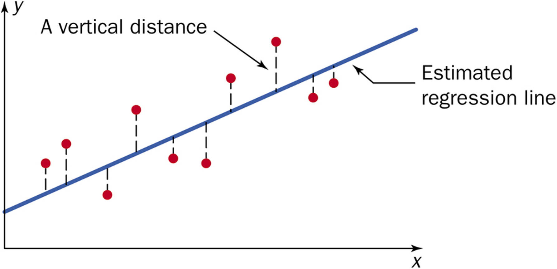
Fig. 13.14 Distances between observed reponses and the fitted line

The goal is mathematically equivalent to finding the arguments that minimize:

(13.2)\[g(\beta_0, \beta_1) = \sum_{i=1}^n (y_i - (\beta_0 + \beta_1 x_i))^2\]

To find their explicit forms, we take the partial derivative of Eq. (13.2) with respect to each parameter and set it equal to zero. Then we solve the resulting system of equations for \(\hat{\beta}_0\) and \(\hat{\beta}_1\).

Derivation of the Intercept Estimate

Take the partial derivative of \(g(\beta_0, \beta_1)\) with respect to \(\beta_0\):

\[\begin{split}\frac{\partial g}{\partial \beta_0} &= \frac{\partial}{\partial \beta_0} \sum_{i=1}^n (y_i - \beta_0 - \beta_1 x_i)^2\\ &= -2 \sum_{i=1}^n (y_i - \beta_0 - \beta_1 x_i)\\ &= \sum_{i=1}^n y_i - n\beta_0 - \beta_1 \sum_{i=1}^n x_i\end{split}\]

By setting this equal to zero and solving for \(\beta_0\), we obtain:

(13.3)\[\hat{\beta}_0 = \frac{1}{n}\sum_{i=1}^n y_i - \beta_1 \frac{1}{n}\sum_{i=1}^n x_i = \bar{y} - \beta_1 \bar{x}.\]

Derivation of the Slope Estimate

Likewise, we take the partial derivative of \(g(\beta_0, \beta_1)\) with respect to \(\beta_1\):

\[\begin{split}\frac{\partial g}{\partial \beta_1} &= -2 \sum_{i=1}^n x_i(y_i - \beta_0 - \beta_1 x_i)\\ &= -2 \left(\sum_{i=1}^n x_i y_i - \beta_0 \sum_{i=1}^n x_i - \beta_1 \sum_{i=1}^n x_i^2 \right)\end{split}\]

Substitute \(\hat{\beta}_0\) (Eq. (13.3)) for \(\beta_0\) and set equal to zero:

\[\begin{split}0 &= \sum_{i=1}^n x_i y_i - (\bar{y}-\beta_1 \bar{x})\sum_{i=1}^n x_i - \beta_1 \sum_{i=1}^n x_i^2\\ &= \sum_{i=1}^n x_i y_i - (\bar{y}-\beta_1 \bar{x})n\bar{x} - \beta_1 \sum_{i=1}^n x_i^2\\ &= \sum_{i=1}^n x_i y_i - n\bar{x}\bar{y} - \beta_1 (\sum_{i=1}^n x_i^2 - n \bar{x}^2)\end{split}\]

Isolate \(\beta_1\) to obtain:

(13.4)\[\hat{\beta}_1 = \frac{\sum_{i=1}^n x_i y_i - n\bar{x}\bar{y}}{\sum_{i=1}^n x_i^2 - n\bar{x}^2}\]

Summary

Slope estimate:

\[\hat{\beta}_1 = \frac{\sum_{i=1}^n x_i y_i - n\bar{x}\bar{y}}{\sum_{i=1}^n x_i^2 - n\bar{x}^2}\]

Intercept estimate:

\[\hat{\beta}_0 = \bar{y} - \hat{\beta}_1 \bar{x}\]

Alternative Notation

The symbols \(b_0\) and \(b_1\) are used interchangeably with \(\hat{\beta}_0\) and \(\hat{\beta}_1\), respectively.

Alternative Expressions of the Slope Estimate

Several alternative expressions exist for the slope estimate \(\hat{\beta}_1\), each offering a different perspective on its relation to various components of regression analysis. Being able to transition freely between these forms is key to deepening the intuition for linear regression and enabling efficient computation.

Define the sum of cross products and the sum of sqaures of \(X\) as:

• \(S_{XY} = \sum_{i=1}^n (x_i - \bar{x})(y_i - \bar{y})\)

• \(S_{XX} = \sum_{i=1}^n (x_i - \bar{x})^2\)

In addition, the sample covariance of \(X\) and \(Y\) is denoted \(s_{XY}\) (lower case \(s\)) and defined as:

\[s_{XY} = \frac{ \sum_{i=1}^n (x_i - \bar{x})(y_i - \bar{y})}{n-1}\]

Also recall that \(s_X^2 = \frac{\sum_{i=1}^n (x_i - \bar{x})^2}{n-1}\) denotes the sample variance of \(x_1, \cdots, x_n\).

Then \(\hat{\beta}_1\) (13.4) can also be written as:

(13.5)\[\hat{\beta}_1 = \frac{S_{XY}}{S_{XX}} = \frac{s_{XY}}{s^2_X} = \frac{\sum_{i=1}^n (x_i -\bar{x})(y_i - \bar{y})}{\sum_{i=1}^n (x_i - \bar{x})^2}\]

Exercise: Prove equality between the alternative expressions

Hint: Showing the second and third equality of (13.5) is relatively simple. To show the first equality, begin with the numerators:

\[\begin{split}\sum_{i=1}^n (x_i -\bar{x})(y_i - \bar{y}) &= \sum_{i=1}^n x_i y_i -\bar{x}\sum_{i=1}^n y_i -\bar{y}\sum_{i=1}^n x_i + n\bar{x}\bar{y}\\ &= \sum_{i=1}^n x_i y_i -\bar{x}(n\bar{y}) -\bar{y}(n\bar{x}) + n\bar{x}\bar{y}\\ &= \sum_{i=1}^n x_i y_i -n\bar{x}\bar{y} \quad ✅\end{split}\]

Repeat a similar procedure for the denominators.

13.2.3. The Fitted Regression Line

Once the slope and intercept estimates are obtained, we can use them to construct the fitted regression line:

\[\hat{y} = \hat{\beta}_0 + \hat{\beta}_1 x.\]

By plugging in specific \(x\) values into the equation, we obtain point estimates of the corresponding responses. The hat notation is essential, as it distinguishes these estimates from the observed responses, \(y\).

Properties of the Fitted Regression Line

1. Interpretation of the Slope

The slope \(\hat{\beta}_1\) represents the estimated average change in the response for every one-unit change in the explanatory variable. The sign of \(\hat{\beta}_1\) indicates the direction of the association.

2. Interpretation of the Intercept

The intercept \(\hat{\beta}_0\) represents the estimated average value of the response when the explanatory variable equals zero. However, this may not have significance if \(X = 0\) is outside the range of the data or not practically meaningful.

3. The Line Passes Through \((\bar{x}, \bar{y})\)

If we substitute \(x = \bar{x}\) into the fitted regression equation:

\[\hat{y} = \hat{\beta}_0 + \hat{\beta}_1\bar{x} = (\bar{y} - \hat{\beta}_1\bar{x}) + \hat{\beta}_1\bar{x} = \bar{y}.\]

That is, a fitted regression line always passes through the point \((\bar{x}, \bar{y})\).

4. Non-exchangeability

If we swap the explanatory and response variables and refit the model, the resulting fitted line will not be the same as the original, nor will the new slope be the algebraic inverse of the original.

Example 💡: Blood Pressure Study

A new treatment for high blood pressure is being assessed for feasibility. In an early trial, 11 subjects had their blood pressure measured before and after treatment. Researchers want to determine if there is a linear association between patient age and the change in systolic blood pressure after 24 hours. Using the data and the summary statistics below, compute and interpret the fitted regression line.

Variable Definitions:

• Explanatory variable (X): Age of patient (years)

• Response variable (Y): Change in blood pressure = (After treatment) - (Before treatment)

Data:

\(i\)	Age (\(x_i\))	ΔBP (\(y_i\))
1	70	-28
2	51	-10
3	65	-8
4	70	-15
5	48	-8
6	70	-10
7	45	-12
8	48	3
9	35	1
10	48	-5
11	30	8

Scatter Plot:

Fig. 13.15 Scatter plot of age vs blood pressure data

Summary Statistics:

• \(n=11\)

• \(\bar{x} = 52.7273\) years

• \(\bar{y} = -7.6364\) mm Hg

• \(\sum x_i y_i = -5485\)

• \(\sum x_i^2 = 32588\)

Slope Calculation:

\[\begin{split}S_{XY} &= \sum x_i y_i - n\bar{x}\bar{y} \\ &= -5485 - 11(52.7273)(-7.6364) \\ &= -1055.8857\\ &\quad\\ S_{XX} &= \sum x_i^2 - n\bar{x}^2\\ &= 32588 - 11(52.7273)^2 \\ &= 2006.1502\end{split}\]

\[b_1 = \frac{S_{xy}}{S_{xx}} = \frac{-1055.8857}{2006.1502} = -0.5263\]

Intercept Calculation:

\[b_0 = \bar{y} - b_1\bar{x} = -7.6364 - (-0.5263)(52.7273) = 20.114\]

Fitted Regression Line:

\[\hat{y} = 20.114 - 0.526x\]

Interpretation:

• For each additional year of age, the change in blood pressure decreases by an average of 0.526 mm Hg.

• The intercept estimate has no practical meaning since we do not study newborns for blood pressure treatment.

• The negative slope suggests that older patients benefit more from the treatment.

---

13.2.4. The ANOVA Table for Regression

Just as in ANOVA, we can decompose the total variability in the response variable into two components, one arising from the model structure and the other from random error.

Total Variability: SST

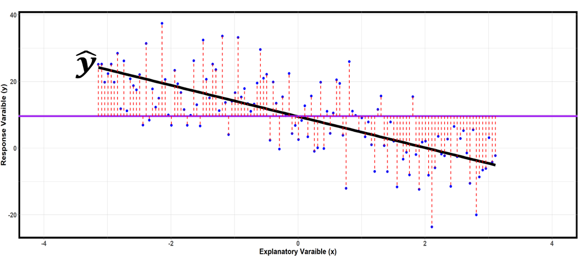
Fig. 13.16 SST is the sum of the squared lengths of all the red dotted lines. They measure the distances of the response values from an overall mean.

(13.6)\[\text{SST} = \sum_{i=1}^n (y_i - \bar{y})^2\]

SST measures how much the response values deviate from their overall mean, ignoring the explanatory variable. SST can also be denoted as \(S_{YY}\). The degrees of freedom associated with \(\text{SST}\) is \(df_T = n-1\).

Computational Shortcut for SST

While Eq. (13.6) conveys its intuitive meaning, it is often more convenient to use the following equivalent formula for computation:

\[\text{SST} = \sum_{i=1}^n y_i^2 - n\bar{y}^2\]

Model Variability: SSR and MSR

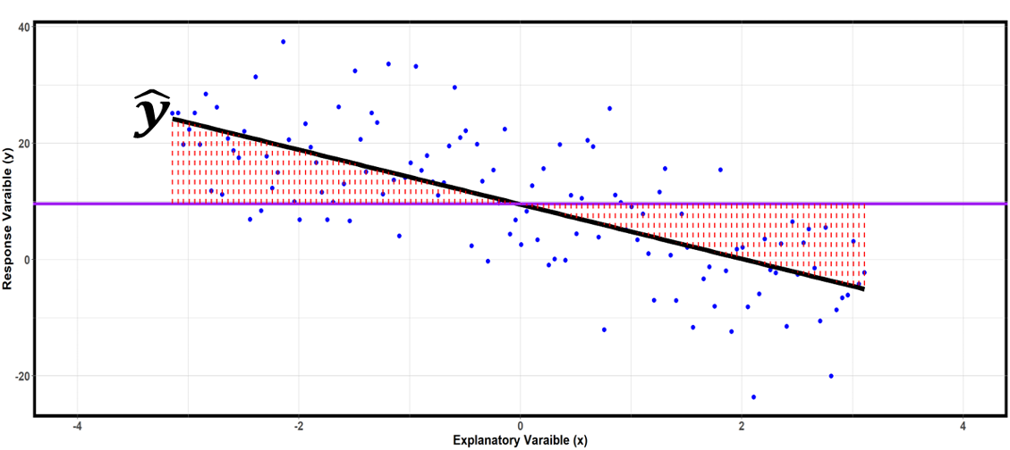
Fig. 13.17 SSR is the sum of the squared lengths of all the red dotted lines. They measure the distances of the predicted \(\hat{y}\) values from an overall mean.

The variability in \(Y\) arising from its linear association with \(X\) is measured with the regression sum of squares, or SSR:

\[\text{SSR} = \sum_{i=1}^n (\hat{y}_i - \bar{y})^2.\]

SSR expresses how much the fitted values deviate from the overall mean. Its associated degrees of freedom is denoted \(df_R\), and it is equal to the number of explanatory variables. In simple linear regression, \(df_R\) is always equal to 1. Therefore,

\[\text{MSR} = \frac{\text{SSR}}{df_R} = \text{SSR}.\]

Computational Shortcut for SSR

Using the expanded formula of \(\hat{y}_i\) and \(\hat{\beta}_0\),

\[\begin{split}\text{SSR} &= \sum_{i=1}^n (\hat{\beta}_0 + \hat{\beta}_1x_i - \bar{y})^2\\ &= \sum_{i=1}^n ((\bar{y}-\hat{\beta}_1\bar{x}) + \hat{\beta}_1x_i - \bar{y})^2\\ &= \hat{\beta}_1^2\sum_{i=1}^n (x_i -\bar{x})^2\\ &= \hat{\beta}_1\frac{S_{XY}}{S_{XX}} S_{XX} = \hat{\beta}_1 S_{XY}\end{split}\]

The final equality uses the definition of \(S_{XX}\) and the fact that \(\hat{\beta}_1 = \frac{S_{XY}}{S_{XX}}\). The resulting equation

\[\text{SSR} = \hat{\beta}_1 S_{XY}\]

is convenient for computaion if \(\hat{\beta}_1\) and \(S_{XY}\) are available.

Variability Due to Random Error: SSE and MSE

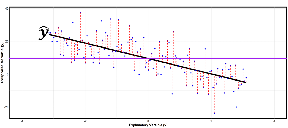
Fig. 13.18 SSE is the sum of the squared lengths of all the red dotted lines. They measure the distances between the observed and predicted response values.

Finally, the variability in \(Y\) arising from random error is measured with the error sum of squares, or SSE:

\[\text{SSE} = \sum_{i=1}^n (y_i - \hat{y}_i)^2 = \sum_{i=1}^n e_i^2\]

The Residuals

Each difference \(e_i = y_i - \hat{y}_i\) is called the \(i\)-th residual. Residuals serve as proxies for the unobserved true error terms \(\varepsilon_i\).

Degrees of Freedom and MSE

The degrees of freedom associated with SSE is \(df_E = n-2\) because its formula involves two estimated parameters (\(b_0\) and \(b_1\)). Readjusting the scale by the degrees of freedom,

\[\text{MSE} = \frac{\text{SSE}}{n-2}.\]

MSE as Variance Estimator

\(\text{MSE}\) is a mean of squared distances of \(y_i\) from their estimated means, \(\hat{y_i}\). Therefore, we use it as an estimator of \(\sigma^2\):

\[\hat{\sigma}^2 = MSE\]

The Fundamental Identity

Just like in ANOVA, the total sum of squares and the total degrees freedom deompose into their respective model and error components:

\[\text{SST} = \text{SSR} + \text{SSE} \quad \text{ and } \quad df_T = df_R + df_E.\]

This can be proven algebraically by adding and subtracting \(\hat{y}_i\) in the expression for SST and using properties of least squares. You are encouraged to show this as an independent exercise.

Partial ANOVA Table for Simple Linear Regression

Source	df	Sum of Squares	Mean Square	F-statistic	p-value
Regression	1	\(\sum_{i=1}^n (\hat{y}_i - \bar{y})^2\)	\(\frac{\text{SSR}}{1}\)	?	?
Error	\(n-2\)	\(\sum_{i=1}^n (y_i - \hat{y}_i)^2\)	\(\frac{\text{SSE}}{n-2}\)
Total	\(n-1\)	\(\sum_{i=1}^n (y_i - \bar{y})^2\)

We will discuss how to compute and use the \(F\)-statistic and \(p\)-value in the upcoming lesson.

Example 💡: Blood Pressure Study, Continued

The summary statistics and the model parameter estimates computed in the previous example for the blood pressure study are listed below:

• \(n=11\)

• \(\bar{x} = 52.7273\) years

• \(\bar{y} = -7.6364\) mm Hg

• \(\sum x_i y_i = -5485\)

• \(\sum x_i^2 = 32588\)

• \(\sum y_i^2 = 1580\)

• \(S_{XY} = -1055.8857\)

• \(S_{XX}=2006.1502\)

• \(b_0 = 20.114\)

• \(b_1 = -0.5263\)

Q1: Predict the change in blood pressure for a patient who is 65 years old. Compute the corresponding residual.

The predicted change is

\[\hat{y} = 20.11 - 0.526(65) = -14.0 \text{ mm Hg}\]

The observed response value for \(x=65\) is \(y=-8\) from the data table. Therefore, the residual is

\[e = -8 - (-14) = 6 \text{ mm Hg}\]

Q2: Complete the ANOVA table for the linear regression model between age and change in blood pressure.

For each sum of squares, we will use the computational shortcut rather than the definition:

\[\begin{split}&\text{SSR} = b_1 S_{xy} = (-0.5263)(-1055.8857) = 555.7126\\ &\text{SST} = \sum y_i^2 - n\bar{y}^2 = 1580 - 11(-7.6364)^2 = 938.5393\end{split}\]

Finally, using the decomposition identity of the sums of squares,

\[\text{SSE} = \text{SST} - \text{SSR} = 938.5393 - 555.7126 = 382.8267\]

The mean squares are:

\[\begin{split}& \text{MSR} = \frac{\text{SSR}}{1} = 555.7126\\ & \text{MSE} = \frac{\text{SSE}}{9} = 42.5363\end{split}\]

The results are organized into a table below:

Source	df	Sum of Squares	Mean Square	F-statistic	p-value
Regression	1	\(555.7126\)	\(555.7126\)	?	?
Error	\(9\)	\(382.8267\)	\(42.5363\)
Total	\(10\)	\(938.5393\)

13.2.5. The Coefficient of Determination (\(R^2\))

The coefficient of determination, denoted \(R^2\), provides a single numerical measure of how well our regression line fits the data. It is defined as:

\[R^2 = \frac{\text{SSR}}{\text{SST}}.\]

Due to the fundamental identity \(\text{SST} = \text{SSR} + \text{SSE}\) and the fact that each component is non-negative, \(R^2\) is always between 0 and 1.

It is interpreted as the fraction of the response variability that is explained by its linear association with the explanatory variable.

\(R^2\) approaches 1 when:

• \(\text{SSR}\) approaches \(\text{SST}\).

• The residuals \(y_i - \hat{y}_i\) have small magnitudes.

• The regression line captures most of the variability in the response.

• Points gather tightly around the fitted line.

\(R^2\) approaches 0 when:

• \(\text{SSE}\) approaches \(\text{SST}\).

• The residuals have large magnitudes.

• The explanatory variable provides little information about the response.

• Points scatter widely around the fitted line.

Example 💡: Blood Pressure Study, Continued

Compute and interpret the coefficient of determination from the blood pressure study.

\[R^2 = \frac{\text{SSR}}{\text{SST}} = \frac{555.7126}{938.5393} = 0.5921\]

Interpretation: Approximately 59.21% of the variation in blood pressure change is explained by the linear relationship with patient age.

Important Limitations of \(R^2\)

While \(R^2\) is a useful summary measure, it has important limitations that require careful interpretation. These limitations are evident in the scatter plots of the well-known Anscome’s quartet (Fig. 13.19). The figure presents four bivariate data sets that have distinct patterns yet are identical in their \(R^2\) values:

Fig. 13.19 Anscome’s Quartet

Let us point out some important observations from Fig. 13.19:

1. A high \(R^2\) value does not guarantee linaer association.

2. \(R^2\) is not robust to outliers. Outliers can dramatically reduce or inflate \(R^2\).

3. A high \(R^2\) does not automatically guarantee good prediction performance.

   • Even when the true form is not linear, we might obtain a high \(R^2\) if the sample size is small and the points happen to align well with a linear pattern.

   • Absolute scale of the observed errors also matter. Consider a scenario where \(\text{SSR} = 9 \times 10^6\) and \(\text{SST} = 10^7\), giving \(R^2 = 0.90\). While 90% of the total variation is explained, \(\text{SSE} = 10^6\) indicates substantial absolute errors that might make predictions unreliable for practical purposes.

Best Practices for Using the Coefficient of Determination

1. Always examine scatter plots to verify model assumptions and check for outliers.

2. Use \(R^2\) as one component of model assessment, not the sole criterion. Consider factors such as sample size, scale, and practical significance.

---

13.2.6. Sample Pearson Correlation Coefficient

Another numerical measure that proves useful in simple linear regression is the sample Pearson correlation coefficient. This provides a standardized quantification of the direction and strength of a linear association. It is defined as:

\[r = \frac{\sum_{i=1}^n (x_i - \bar{x})(y_i - \bar{y})}{\sqrt{\sum_{i=1}^n (x_i - \bar{x})^2} \sqrt{\sum_{i=1}^n (y_i - \bar{y})^2}}.\]

As suggested by the structural similarity, \(r\) is the sample equivalent of the population correlation introduced in the probability chapters:

(13.7)\[\rho = \frac{E[(X - \mu_X)(Y - \mu_Y)]}{\sigma_X \sigma_Y}.\]

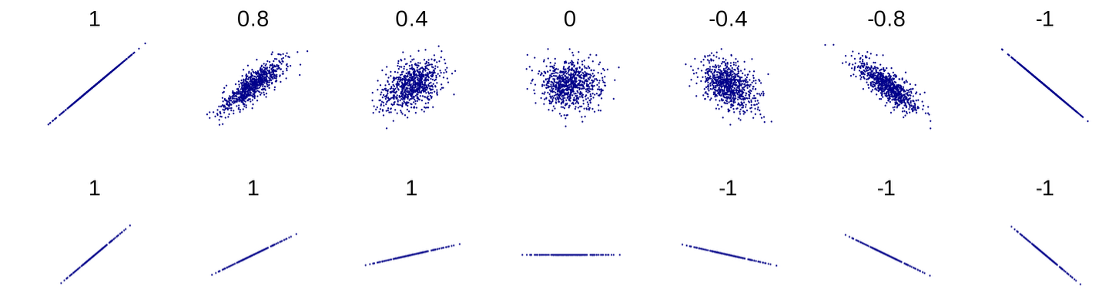
Fig. 13.20 Scatter plots with different sample correlation values

Sample correlation is unitless and always falls between -1 and +1, with the sign indicating the direction and the magnitude indicating the strength of linear association. The bounded range makes it easy to compare correlations across different data sets.

We classify linear associations as strong, moderate or weak using the following rule of thumb:

• Strong association: \(0.8 <|r| \leq 1\)

• Moderate association: \(0.5 <|r| \leq 8\)

• Weak association: \(0 \leq |r| \leq 0.5\)

Alternative Expressions of Sample Correlation

1. Using Sample Covariance and Sample Standard Deviations

Using the sample covariance \(s_{XY} = \frac{1}{n-1}\sum_{i=1}^n(x_i-\bar{x})(y_i-\bar{y})\) and the sample standard deviations \(s_X\) and \(s_Y\), we can rewrite the definition of sample correlation (13.7) as:

(13.8)\[r = \frac{s_{XY}}{s_X s_Y}.\]

This definition gives us an insight into what \(r\) measures. Sample covariance is an unscaled measure of how \(X\) and \(Y\) move together.

• If the two variables typically take values above or below their respective means simultaneously, most terms in the summation will be positive, increasing the chance that the mean of these terms, the sample covariance, is also positive.

• If the values tend to lie on opposite sides of their respective means, the sample covariance is likely negative.

Sample correlation is obtained by removing variable-specific scales from sample covariance, dividing it by the sample standard deviations of both \(X\) and \(Y\).

2. Using Sums of Cross-products and Squares

The definition of sample correlation can also be expressed using the sums of cross-products and squares, \(S_{XY}, S_{XX},\) and \(S_{YY}\):

\[r = \frac{S_{XY}}{\sqrt{S_{XX}S_{YY}}}.\]

3. Cross-products of Standardized Data

Modifying the equation (13.8),

\[\begin{split}r &= \frac{\sum_{i=1}^n[(x_i - \bar{x})(y_i - \bar{y})]/(n-1)}{s_X s_Y}\\ &= \frac{1}{n-1}\sum_{i=1}^n \left(\frac{x_i - \bar{x}}{s_X}\right)\left(\frac{y_i - \bar{y}}{s_Y}\right).\end{split}\]

This gives us another perspective into what the correlation coefficient is really doing—it is a mean of cross-products of the standardized values of the explanatory and response variables.

Connections with Other Components of Linear Regression

1. Slope Estimate, \(b_1\)

Both the correlation coefficient and the slope estimate capture information about a linear relationship. How exactly are they connected?

Recall that one way to write the slope estimate is:

\[b_1 = \frac{s_{XY}}{s_X^2}.\]

Using the correlation formula \(r = \frac{s_{XX}}{s_X s_Y}\), the slope estimate can be written as:

\[b_1 = \frac{r s_X s_Y}{s_X^2} = r \frac{s_Y}{s_X}\]

This relationship shows that the slope estimate is simply the correlation coefficient rescaled by the ratio of standard deviations.

2. Coefficient of Determination, \(R^2\)

Recall that:

• \(b_1 = \frac{S_{XY}}{S_{XX}}\)

• \(\text{SSR} = b_1 S_{XY}\)

• \(\text{SST} = S_{YY}\)

Combining these together,

\[R^2 = \frac{\text{SSR}}{\text{SST}} = \frac{b_1 S_{XY}}{S_{YY}} = \frac{S_{XY}^2}{S_{XX}S_{YY}} = \left(\frac{S_{XY}}{\sqrt{S_{XX} S_{YY}}}\right)^2 = r^2.\]

In other words, the coefficient of determination is equal to the square of the correlation coefficient. However, this special relationship holds only for simple linear regression, where the model has a single explanatory variable.

Limitations of Correlation

Correlation specifically measures the direction and strength of linear association. Therefore, \(r = 0\) indicates an absence of linear association, not necessarily an absence of association altogether. Symmetrical non-linear relationships tend to produce sample correlation close to zero, as any linear trend one one side offsets the trend on the other.

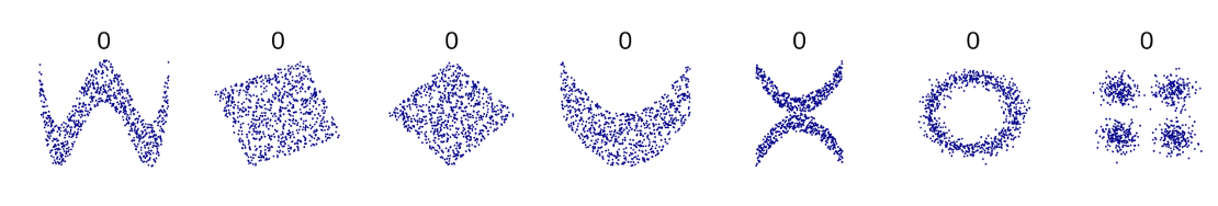
Fig. 13.21 Scatter plots with zero sample correlation

Furthermore, extreme observations can significantly impact correlation values. These limitations mean we need to examine our data visually before trusting correlation values, just as we do with \(R^2\).

13.2.7. Bringing It All Together

Key Takeaways 📝

1. The simple linear regression model \(Y_i = \beta_0 + \beta_1 x_i + \varepsilon_i\) and its associated assumptions formalize the linear relationship between quantitative variables.

2. The least squares method provides optimal estimates for the slope and intercept parameters by minimizing the sum of squared differences between the observed data and the summary line.

3. The variability components of linear regression can also be organized into an ANOVA table.

4. Residuals \(e_i = y_i - \hat{y}_i\) estimate the unobserved error terms and enable variance estimation through \(s^2 = \text{MSE} = \text{SSE}/(n-2)\).

5. The coefficient of determination \(R^2 = \text{SSR}/\text{SST}\) measures the proportion of total variation in observed \(Y\) that is explained by the regression model.

6. The sample Pearson correlation coefficient \(r\) provides the direction and strength of a linear relationship on a standard numerical scale between -1 and 1.

7. Model assessment requires multiple tools: scatter plots, residual analysis, ANOVA table, \(R^2\), and \(r\) all work together to evaluate model appropriateness.

13.2.8. Exercises

Exercise 1: Least Squares Calculation

An aerospace engineer is studying the relationship between altitude (X, in thousands of feet) and air density (Y, in kg/m³) for aircraft performance modeling. The following data were collected:

Altitude (000 ft)	Air Density (kg/m³)
0	1.225
5	1.056
10	0.905
15	0.771
20	0.653
25	0.549

Given summary statistics:

• \(n = 6\), \(\bar{x} = 12.5\), \(\bar{y} = 0.8598\)

• \(\sum x_i = 75\), \(\sum y_i = 5.159\)

• \(\sum x_i^2 = 1375\), \(\sum x_i y_i = 52.68\)

1. Calculate \(S_{XX}\) and \(S_{XY}\).

2. Calculate the least squares estimate of the slope \(b_1\).

3. Calculate the least squares estimate of the intercept \(b_0\).

4. Write the fitted regression equation.

5. Interpret the slope in context.

6. Interpret the intercept in context. Is it meaningful?

Solution

Part (a): Calculate S_XX and S_XY

\[S_{XX} = \sum x_i^2 - n\bar{x}^2 = 1375 - 6(12.5)^2 = 1375 - 937.5 = 437.5\]

\[S_{XY} = \sum x_i y_i - n\bar{x}\bar{y} = 52.68 - 6(12.5)(0.8598) = 52.68 - 64.485 = -11.805\]

Part (b): Slope estimate

\[b_1 = \frac{S_{XY}}{S_{XX}} = \frac{-11.805}{437.5} = -0.02699\]

Part (c): Intercept estimate

\[b_0 = \bar{y} - b_1\bar{x} = 0.8598 - (-0.02699)(12.5) = 0.8598 + 0.3374 = 1.1972\]

Part (d): Fitted equation

\(\hat{y} = 1.1972 - 0.02699x\)

Or in context: Air Density = 1.1972 − 0.02699(Altitude)

Part (e): Slope interpretation

For each additional 1,000 feet of altitude, air density decreases by approximately 0.027 kg/m³.

Part (f): Intercept interpretation

At sea level (altitude = 0), the predicted air density is 1.1972 kg/m³. This is meaningful and very close to the actual sea level air density of 1.225 kg/m³, so the intercept has a valid physical interpretation.

R verification:

alt <- c(0, 5, 10, 15, 20, 25)
density <- c(1.225, 1.056, 0.905, 0.771, 0.653, 0.549)
fit <- lm(density ~ alt)
coef(fit)  # Intercept: 1.197, alt: -0.02699

---

Exercise 2: Properties of Least Squares Line

Using the air density regression from Exercise 1:

1. Verify that the fitted line passes through \((\bar{x}, \bar{y})\).

2. Calculate the predicted air density at 12,000 feet (x = 12).

3. Calculate the residual for the observation at 10,000 feet (x = 10, y = 0.905).

4. What is the sum of all residuals for a least squares regression line? Explain why.

Solution

Part (a): Verification

At \(x = \bar{x} = 12.5\):

\(\hat{y} = 1.1972 - 0.02699(12.5) = 1.1972 - 0.3374 = 0.8598 = \bar{y}\) ✓

The fitted line passes through the point \((\bar{x}, \bar{y}) = (12.5, 0.8598)\).

Part (b): Prediction at x = 12

\(\hat{y} = 1.1972 - 0.02699(12) = 1.1972 - 0.3239 = 0.8733\) kg/m³

Part (c): Residual at x = 10

First, calculate the fitted value:

\(\hat{y} = 1.1972 - 0.02699(10) = 1.1972 - 0.2699 = 0.9273\)

Then the residual:

\(e = y - \hat{y} = 0.905 - 0.9273 = -0.0223\)

The negative residual indicates the observed value is slightly below the fitted line.

Part (d): Sum of residuals

The sum of all residuals for a least squares line is always zero (or essentially zero due to rounding).

This is a mathematical property of the least squares method: the normal equations guarantee that \(\sum_{i=1}^{n} e_i = 0\). Geometrically, the line passes through \((\bar{x}, \bar{y})\), causing positive and negative residuals to balance exactly.

---

Exercise 3: ANOVA Table Construction

A chemical engineer studies the relationship between reaction temperature (°C) and product yield (%). With \(n = 15\) observations, the regression analysis yields:

• \(\bar{y} = 72.4\)

• \(b_0 = 35.2\), \(b_1 = 0.62\)

• \(SST = \sum_{i=1}^{15}(y_i - \bar{y})^2 = 2450\)

• \(SSR = \sum_{i=1}^{15}(\hat{y}_i - \bar{y})^2 = 1862\)

1. Calculate SSE using the relationship SST = SSR + SSE.

2. Complete the ANOVA table with all degrees of freedom, sums of squares, mean squares, and F-statistic.

3. Calculate the estimate of \(\sigma\) (the standard deviation of errors).

4. Calculate \(R^2\) and interpret its meaning in context.

Solution

Part (a): Calculate SSE

\(SSE = SST - SSR = 2450 - 1862 = 588\)

Part (b): Complete ANOVA table

Source	df	SS	MS	F
Regression	1	1862	1862.00	41.17
Error	13	588	45.23
Total	14	2450

Calculations:

• \(df_{Reg} = 1\) (simple linear regression)

• \(df_{Error} = n - 2 = 15 - 2 = 13\)

• \(df_{Total} = n - 1 = 14\)

• \(MSR = SSR/df_{Reg} = 1862/1 = 1862\)

• \(MSE = SSE/df_{Error} = 588/13 = 45.23\)

• \(F = MSR/MSE = 1862/45.23 = 41.17\)

Part (c): Estimate of σ

\(\hat{\sigma} = \sqrt{MSE} = \sqrt{45.23} = 6.725\)

This estimates the standard deviation of the random errors around the regression line.

Part (d): R² and interpretation

\(R^2 = \frac{SSR}{SST} = \frac{1862}{2450} = 0.76 = 76\%\)

Interpretation: Approximately 76% of the variation in product yield is explained by the linear relationship with reaction temperature.

---

Exercise 4: Coefficient of Determination

For each scenario, interpret what the given \(R^2\) value means:

1. A regression of fuel consumption (mpg) on vehicle weight (lbs) yields \(R^2 = 0.78\).

2. A regression of exam score on hours of study yields \(R^2 = 0.35\).

3. A regression of chip manufacturing yield on equipment age yields \(R^2 = 0.95\).

4. Which regression model would you be most confident using for predictions? Least confident? Explain.

Solution

Part (a): Fuel consumption model (R² = 0.78)

78% of the variation in fuel consumption is explained by the linear relationship with vehicle weight. This is a reasonably strong model—weight is an important predictor of fuel efficiency.

Part (b): Exam score model (R² = 0.35)

Only 35% of the variation in exam scores is explained by hours of study. This suggests that while study time helps, many other factors (prior knowledge, test-taking ability, sleep, etc.) affect scores.

Part (c): Chip yield model (R² = 0.95)

95% of the variation in manufacturing yield is explained by equipment age. This is a very strong relationship, indicating equipment age is the dominant factor affecting yield.

Part (d): Confidence in predictions

• Most confident: Chip manufacturing yield model (\(R^2 = 0.95\)) — predictions will have the smallest prediction errors since almost all variation is explained.

• Least confident: Exam score model (\(R^2 = 0.35\)) — predictions will have large uncertainty since 65% of variation is unexplained.

Higher \(R^2\) means less unexplained variation, leading to more precise predictions.

---

Exercise 5: Relationship Between r and R²

For a simple linear regression of server response time (Y, ms) on number of concurrent users (X):

• Sample correlation: \(r = -0.82\)

1. Calculate \(R^2\).

2. What percentage of the variation in response time is explained by the number of users?

3. What percentage is unexplained (due to other factors)?

4. What is the sign of the slope \(b_1\)? How do you know?

Solution

Part (a): Calculate R²

\(R^2 = r^2 = (-0.82)^2 = 0.6724\)

Part (b): Explained variation

67.24% of the variation in response time is explained by the linear relationship with number of concurrent users.

Part (c): Unexplained variation

\(1 - R^2 = 1 - 0.6724 = 0.3276 = 32.76\%\) is unexplained.

This variation is due to other factors like server configuration, network latency, query complexity, etc.

Part (d): Sign of slope

The slope \(b_1\) is negative.

We know this because \(r = -0.82 < 0\), and the slope and correlation always have the same sign. This makes sense: more concurrent users typically increase (not decrease) response time, so there may be an error in the problem setup—or this represents a scenario where more users triggers server scaling.

Note: If the negative correlation seems counterintuitive, it could represent a scenario where higher traffic triggers auto-scaling or caching improvements.

---

Exercise 6: Residual Analysis Basics

A materials scientist models tensile strength (MPa) as a function of carbon content (%) in steel alloys. The regression output gives \(\hat{y} = 280 + 450x\).

For the following observations, calculate the fitted value and residual:

Carbon Content (x)	Tensile Strength (y)	Fitted Value (\(\hat{y}\))	Residual (\(e\))
0.20	365	?	?
0.35	445	?	?
0.50	520	?	?
0.65	570	?	?

1. Complete the table above.

2. What does a positive residual indicate about the observed vs. predicted value?

3. What does a negative residual indicate?

Solution

Part (a): Completed table

Carbon Content (x)	Tensile Strength (y)	Fitted Value (\(\hat{y}\))	Residual (\(e\))
0.20	365	370	−5
0.35	445	437.5	+7.5
0.50	520	505	+15
0.65	570	572.5	−2.5

Calculations:

• \(\hat{y}_{0.20} = 280 + 450(0.20) = 280 + 90 = 370\)

• \(\hat{y}_{0.35} = 280 + 450(0.35) = 280 + 157.5 = 437.5\)

• \(\hat{y}_{0.50} = 280 + 450(0.50) = 280 + 225 = 505\)

• \(\hat{y}_{0.65} = 280 + 450(0.65) = 280 + 292.5 = 572.5\)

Part (b): Positive residual

A positive residual (\(e > 0\)) indicates the observed value is above the regression line—the actual tensile strength is higher than predicted by the model.

Part (c): Negative residual

A negative residual (\(e < 0\)) indicates the observed value is below the regression line—the actual tensile strength is lower than predicted by the model.

---

Exercise 7: MSE and Standard Error

From an ANOVA table for a regression with \(n = 20\) observations:

• SSE = 324

• SSR = 1296

1. Calculate the degrees of freedom for error.

2. Calculate MSE.

3. Calculate the estimate of \(\sigma\).

4. What does this estimate of \(\sigma\) represent in the context of the regression model?

Solution

Part (a): Degrees of freedom for error

\(df_{Error} = n - 2 = 20 - 2 = 18\)

Part (b): MSE

\(MSE = \frac{SSE}{df_{Error}} = \frac{324}{18} = 18\)

Part (c): Estimate of σ

\(\hat{\sigma} = \sqrt{MSE} = \sqrt{18} = 4.243\)

Part (d): Interpretation

The estimate \(\hat{\sigma} = 4.243\) represents the estimated standard deviation of the random errors (\(\varepsilon_i\)) in the regression model.

In practical terms:

• It measures the typical vertical distance of data points from the regression line

• It quantifies the “noise” or unexplained variation in Y after accounting for X

• Smaller values indicate data points cluster more tightly around the fitted line

---

Exercise 8: Alternative Slope Formulas

The slope estimate can be written in multiple equivalent forms:

\[b_1 = \frac{S_{XY}}{S_{XX}} = \frac{\sum(x_i - \bar{x})(y_i - \bar{y})}{\sum(x_i - \bar{x})^2} = r \cdot \frac{s_Y}{s_X}\]

Given:

• \(r = 0.85\)

• \(s_X = 12.4\) (standard deviation of X)

• \(s_Y = 28.6\) (standard deviation of Y)

1. Calculate \(b_1\) using the formula \(b_1 = r \cdot \frac{s_Y}{s_X}\).

2. If the correlation changed to \(r = -0.85\) (same magnitude, opposite sign), what would \(b_1\) be?

3. What does this relationship tell us about the connection between correlation and slope?

Solution

Part (a): Calculate b₁

\[b_1 = r \cdot \frac{s_Y}{s_X} = 0.85 \times \frac{28.6}{12.4} = 0.85 \times 2.306 = 1.960\]

Part (b): With negative correlation

\[b_1 = (-0.85) \times \frac{28.6}{12.4} = -0.85 \times 2.306 = -1.960\]

Part (c): Connection between r and b₁

Key relationships:

1. Same sign: The slope and correlation always have the same sign. Positive r means positive slope; negative r means negative slope.

2. Magnitude relationship: The slope magnitude depends on both |r| and the ratio of standard deviations (sY/sX).

3. Scaling: A steeper slope doesn’t necessarily mean stronger correlation—it could just mean Y has larger spread relative to X.

4. Interpretation: Correlation measures strength of linear association on a standardized scale (−1 to 1), while slope measures the actual rate of change in Y per unit change in X (in original units).

---

Exercise 9: Model Assumptions Conceptual

The simple linear regression model is \(Y_i = \beta_0 + \beta_1 x_i + \varepsilon_i\) where \(\varepsilon_i \stackrel{iid}{\sim} N(0, \sigma^2)\).

For each statement, identify which assumption(s) would be violated:

1. The relationship between X and Y follows a curved pattern.

2. The spread of Y values around the regression line increases as X increases.

3. The data were collected over time and consecutive observations tend to have similar residuals.

4. Several residuals have extremely large magnitudes compared to others.

5. Observations were randomly selected and there is no connection between different data points.

Solution

Part (a): Curved pattern

Violates Linearity — The model assumes \(E[Y|X] = \beta_0 + \beta_1 X\) is a straight line. A curved pattern means this assumption fails.

Part (b): Spread increases with X

Violates Equal Variance (Homoscedasticity) — The model assumes \(Var(\varepsilon_i) = \sigma^2\) is constant for all observations. Increasing spread (funnel shape) indicates heteroscedasticity.

Part (c): Consecutive observations have similar residuals

Violates Independence — The “iid” assumption requires errors to be independent. When consecutive observations are correlated (autocorrelation), this assumption fails. Common in time series data.

Part (d): Extreme residuals

Potentially violates Normality — While outliers don’t necessarily violate assumptions (they could be legitimate extreme values from a normal distribution), multiple extreme residuals suggest the errors may not follow a normal distribution (e.g., heavy-tailed distribution).

Part (e): Random selection, no connection

This describes a situation where no assumptions are violated — this is exactly what the independence assumption requires.

---

13.2.9. Additional Practice Problems

Quick Calculations

1. Given \(\sum x_i^2 = 500\), \(n = 10\), \(\bar{x} = 6\), calculate \(S_{XX}\).

2. If \(b_1 = 2.5\), \(\bar{x} = 10\), and \(\bar{y} = 40\), find \(b_0\).

3. SST = 1000, SSR = 750. Calculate SSE and \(R^2\).

True/False

4. The least squares line minimizes the sum of squared horizontal distances from points to the line.

5. If \(R^2 = 1\), then SSE = 0.

6. The residuals from a least squares fit always sum to zero.

Answers to Practice Problems

Quick Calculations:

1. \(S_{XX} = \sum x_i^2 - n\bar{x}^2 = 500 - 10(6)^2 = 500 - 360 = 140\)

2. \(b_0 = \bar{y} - b_1\bar{x} = 40 - 2.5(10) = 40 - 25 = 15\)

3. \(SSE = SST - SSR = 1000 - 750 = 250\); \(R^2 = SSR/SST = 750/1000 = 0.75\)

True/False:

4. FALSE — Least squares minimizes the sum of squared vertical distances (residuals), not horizontal distances.

5. TRUE — If \(R^2 = 1\), then \(SSR = SST\), so \(SSE = SST - SSR = 0\). All points lie exactly on the regression line.

6. TRUE — This is a mathematical property of the least squares method. The normal equations guarantee \(\sum e_i = 0\).