Slides 📊

Download Chapter 11 slides (PPTX)

11.5. Paired Two-Sample Analysis

Researchers often encounter situations where observations are naturally paired in practice. Such dependence requires a revised statistical framework to ensure valid inference.

Road Map 🧭

• Formulate a paired two-sample problem as a single-sample problem of differences, and recognize the structural similarities of the analaysis with the one-sample methods.

• Be aware of the consequences of incorrectly using paired versus independent two-sample methods.

11.5.1. Characteristics of Paired Observations

Paired-sample procedures are appropriate when observations are linked by underlying characteristics that create dependence between measurements. These links can arise through several mechanisms:

• Before-and-after studies where each subject is measured twice, before and after a treatment is applied.

• Pairing subjects based on shared characteristics such as age, gender, and diseases severity.

• Applying different treatments to two pieces from the same source (also called the split-plot design). Examples include sub-plots of crops, pieces cut from the same fabric, and metal from the same alloy.

Pairing is particularly valuable when the extraneous characteristics that link the observations create large variability that might otherwise obscure the treatment effect. By focusing only on the within-pair differences, we eliminate the influence of individual variation from the analysis result.

11.5.2. Notation and Assumptions

We begin with a review of the notation for paired two-sample analyses, first introduced in Chapter 11.1.4.

Observations from Population A and B are denoted \(X_{A1}, X_{A2}, \ldots, X_{An}\) and \(X_{B1}, X_{B2}, \ldots, X_{Bn}\), respectively. The observations are ordered so that \(X_{Ai}\) is paired with \(X_{Bi}\) for each \(i\).

Define the pair-wise differences as:

\[D_i = X_{Ai} - X_{Bi} \text{ for } i = 1, 2, \ldots, n.\]

The validity of paired two-sample procedures rests on the following three fundamental assumptions. They must be carefully verified before applying the inference methods introduced in this lessson.

Assumption 1. Independence between pairs

Each pair \((X_{Ai}, X_{Bi})\) must be independent of all other pairs \((X_{Aj}, X_{Bj})\) for \(i \neq j\).

Distinguish within-pair and between-pair independence

This assumption pertains solely to the independence of pairs across the sample; it does not make any claim about the form or strength of association that may exist within individual pairs.

Assumption 2. Simple Random Sample of Pairs

The pairs must constitute a simple random sample from the population of potential pairs. Combined with Assumption 1, this ensures that the bivariate random variables \((X_{A1}, X_{B1}), (X_{A2}, X_{B2}), \cdots, (X_{An}, X_{Bn})\) form an iid sample of the population of all possible pairs.

This also implies that the pair-wsie differences \(D_1, D_2, \cdots, D_n\) are iid.

Assumption 3. Normality of Differences

The differences \(D_i\) must be normally distributed, or the sample size must be large enough for the Central Limit Theorem to ensure that \(\bar{D}\) is approximately normally distributed.

Note that this assumption concerns the distribution of differences, not the original observations.

11.5.3. The Population Parameter and Its Point Estimator

The Population Mean of Differences

The novelty of the paired two-sample procedure is that it analyzes the distribution of individual differences. Therefore, the central population parameter is \(\mu_D\), the true mean of all possible differences.

In fact, however, the point value of \(\mu_D\) is equal to \(\mu_A - \mu_B\), the central parameter of the independent two-sample procedure.

\[\mu_D = E[D_i] = E[X_{Ai} - X_{Bi}] = E[X_{Ai}] - E[X_{Bi}] = \mu_A - \mu_B\]

This may at first obscure the difference between the two methods, but the key distinction arises in how the population variance of the differences is defined.

The Population Variacnce of Differences

Using the properties of variance for correlated random variables:

\[\begin{split}\sigma^2_D &= \text{Var}[D_i]\\ &= \text{Var}[X_{Ai}] + \text{Var}[X_{Bi}] - 2\text{Cov}[X_{Ai}, X_{Bi}]\\ &= \sigma^2_A + \sigma^2_B - 2\sigma_A\sigma_B\rho_{AB}\end{split}\]

The true variance of the differences now contains an additional term \(- 2\sigma_A\sigma_B\rho_{AB}\).

While we could theoretically estimate the components \(\sigma^2_A, \sigma^2_B,\) and \(\rho_{AB},\) individually, this approach would be unnecessarily complex. Instead, the transformation of data from two samples to a single list of differences allows us to estimate \(\sigma^2_D\) directly using \(S_D^2\), then apply the familiar one-sample \(t\)-procedures.

11.5.4. The Point Estimator and Its Distribution

Sample Mean of Differences

The sample mean of differences provides an ubiased point estimator for \(\mu_D\):

\[\bar{D} = \frac{1}{n}\sum_{i=1}^n D_i = \frac{1}{n}\sum_{i=1}^n (X_{Ai} - X_{Bi}) = \bar{X}_A - \bar{X}_B\]

Note that the point value of an observed mean of differences \(\bar{d}\) is also identical to the observed difference of the two means \(\bar{x}_A - \bar{x}_B\).

Sampling Distribution of \(\bar{D}\)

Under the assumptions listed in Section 11.5.2 above,

\[\bar{D} \sim N\left(\mu_D, \frac{\sigma_D}{\sqrt{n}}\right).\]

Sample Variance of Differences

The sample variance of differences \(S^2_D\) is calculated using the standard formula applied to the differences:

\[S^2_D = \frac{1}{n-1}\sum_{i=1}^n (D_i - \bar{D})^2.\]

This provides an unbiased estimator for \(\sigma^2_D\).

11.5.5. Hypothesis Testing for Paired Samples

Paired sample hypothesis testing follows the same four-step framework as one-sample procedures, but with careful attention to defining the differences appropriately.

Step 1: Parameter Identification and Difference Definition

The parameter of interest is \(\mu_D\), the mean difference between paired observations. Critically, we must explicitly define how the difference is calculated, as this determines the direction of our alternative hypothesis.

For example, if studying a training program’s effectiveness by comparing pre-test and post-test scores, we can define the difference \(D\) as either:

• \(D = X_{\text{pre}} - X_{\text{post}}\), or

• \(D = X_{\text{post}} - X_{\text{pre}}\).

The choice should align with the research question and the anticipated direction of the effect.

Step 2: Hypothesis Formulation

The three types of possible hypothesis pairs are:

Upper-Tailed Hypothesis Test

\[\begin{split}&H_0: \mu_D \leq \Delta_0\\ &H_a: \mu_D > \Delta_0\end{split}\]

Lower-Tailed Hypothesis Test

\[\begin{split}&H_0: \mu_D \geq \Delta_0\\ &H_a: \mu_D < \Delta_0\end{split}\]

Two-Tailed Hypothesis Test

\[\begin{split}&H_0: \mu_D = \Delta_0\\ &H_a: \mu_D \neq \Delta_0\end{split}\]

The choice should reflect how we defined the differences in Step 1.

Step 3: Test Statistic and P-Value Calculation

The test statistic follows the familiar one-sample \(t\)-test format:

\[T_{TS} = \frac{\bar{D} - \Delta_0}{S_d/\sqrt{n}}\]

Under the null hypothesis and the stated assumptions, the test statistic follows a \(t\)-distribution with \(df = n - 1\). \(p\)-value calculation follows the same patterns as one-sample procedures:

\(p\)-Values for paired two-sample \(t\)-Test
Upper-tailed	\[P(T_{n-1} \geq t_{TS})\] tts <- (dbar-delta0)/(s_d/sqrt(n)) pt(tts, df=n-1, lower.tail=FALSE)
Lower-tailed	\[P(T_{n-1} \leq t_{TS})\] pt(tts, df=n-1)
Two-tailed	\[2P(T_{n-1} \leq -|t_{TS}|) \quad \text{ or } \quad 2P(T_{n-1} \geq |t_{TS}|)\] 2 * pt(-abs(tts), df=n-1) 2 * pt(abs(tts), df=n-1, lower.tail=FALSE)

Step 4: Decision and Conclusion

Compare the \(p\)-value to the predetermined significance level \(\alpha\) and draw conclusions in the context of the original research question, being careful to interpret results in terms of the mean difference as defined in Step 1.

Example 💡: Nursing Sensitivity Training Study

A regional hospital conducted a study to determine whether sensitivity training would improve the quality of care provided by their nursing staff. Eight nurses were selected, and their nursing skills were evaluated on a scale from 1 to 10, where higher scores indicate greater sensitivity to patients. After this initial assessment, the nurses participated in a training program, and their skills were evaluated again using the same scale.

Perform a hypothesis test at \(\alpha=0.01\) to determine if the training improves the quality of care provided by the nursing staff.

Step 0: Analysis of Data & Background Information

Since each nurse serves as their own control (measured before and after training), this is clearly a paired design. The data shows pre-training scores, post-training scores, and the calculated differences for each nurse:

ID	Pre-Training	Post-Training	Difference (Pre - Post)
1	2.56	4.54	1.98
2	3.22	5.33	-2.11
3	3.45	4.32	0.87
4	5.55	7.45	1.90
5	5.63	7.00	1.37
6	7.89	9.80	1.91
7	7.66	7.33	0.33
8	6.20	6.80	0.60
Sample mean	\(\bar{x}_{pre} = 5.27\)	\(\bar{x}_{post} = 6.57\)	\(\bar{d} = -1.30\)
Sample sd	\(s_{pre} = 2.018\)	\(s_{post} = 1.803\)	\(s_d = 0.8608\)

Step 1: Parameter Identification

The parameter of interest is \(\mu_D\), the true mean difference between pre-training and post-training nursing sensitivity scores. Using the same order as the data table, define the difference as \(D = X_{\text{pre}} - X_{\text{post}}\).

Step 2: Hypothesis Formulation

Increase in the score corresponds to a negative value for \(\mu_D\) as defined in Step 1. Therefore, we perform a lower-tailed hypothesis test:

\[\begin{split}&H_0: \mu_D \geq 0\\ &H_a: \mu_D < 0\end{split}\]

Step 3: Test Statistic, degrees of freedom, and p-Value

The observed test statistic is:

\[t_{TS} = \frac{\bar{d} - \Delta_0}{s_d/\sqrt{n}} = \frac{-1.30 - 0}{0.8608/\sqrt{8}} = \frac{-1.30}{0.3044} = -4.2755\]

Under the assumptions and the null hypothesis, this value would have been generated from a \(t\)-distributed random variable with \(df = n - 1 = 7\).

For a lower-tailed test, the \(p\)-value is \(p = P(T_7 < -4.2755) = 0.001838\).

Step 4: Decision and Conclusion

Since p-value \(= 0.001838 < \alpha = 0.01\), we reject the null hypothesis. The data gives strong support (p-value \(= 0.001838\)) to the claim that the population average nursing sensitivity score improves after the training.

11.5.6. Confidence Regions for Paired Differences

The \((1-\alpha)100 \%\) confidence regions follow the same format as the standard one-sample case:

Confidence regions for the mean of differences (paired two-sample procedure)
Confidence Interval	\[\bar{d} \pm t_{\alpha/2, n-1} \cdot \frac{s_d}{\sqrt{n}}\]
Upper Confidence Bound	\[\bar{d} + t_{\alpha, n-1} \cdot \frac{s_d}{\sqrt{n}}\]
Lower Confidence Bound	\[\bar{d} - t_{\alpha, n-1} \cdot \frac{s_d}{\sqrt{n}}\]

Example 💡: Nursing Sensitivity Training Study

For the study on the sensitivity score of nursing staff before and after training, compute the \(99\%\) confidence region which provides consistent results with the previous hypothesis test. Explain how the two inferences agree with each other.

The Confidence Region

Since we conducted a left-tailed test, the corresponding confidence bound is an upper bound. The critical value is \(t_{0.01,7} = 2.998\). Putting the components together,

\[UCB = -1.30 + 2.998 \times \frac{0.8608}{\sqrt{8}} = -1.30 + 0.913 = -0.387.\]

We are 99% confident that the true mean difference between pre- and post-training scores is less than -0.387.

Does It Align with the Hypothesis Test?

Since this upper bound is negative (the region does not include the null value \(\Delta_0= 0\)), it confirms that the training program produces improvement.

Simultaneous R Implementation of Confidence Region and Hypothesis Testing

🛑 This approach works only if you have access to the raw data. If the summary statistics are provided instead, solve the problem by substituting appropriate values to an appropriate formula as shown above and in the previous example.

# Define the data
pre_training <- c(2.56, 3.22, 3.45, 5.55, 5.63, 7.89, 7.66, 6.20)
post_training <- c(4.54, 5.33, 4.32, 7.45, 7.00, 9.80, 7.33, 6.80)

# Perform paired t-test
t.test(pre_training, post_training,
      mu = 0,
      conf.level = 0.99,
      paired = TRUE,
      alternative = "less")

11.5.7. Importance of Using the Correct Analysis Method

The choice between paired and independent two-sample procedures depends on the study design and data structure. Making the wrong choice can lead to invalid inference or substantial loss of statistical power.

Using Paired Design When Independence Holds

If we use a paired design on populations which are in fact independent, we face two kinds of losses.

1. Experimental resources: We may waste time or expenses trying to find a good pair for each participant and taking measures against subject dropouts or carryover effects, when these steps are not necessary.

2. Reduced degrees of freedom: When \(n=n_A = n_B\), the paired method gives \(df=n-1\), while the pooled independent two-sample method gives \(df=n_A + n_B - 2\). By incorrectly using the paired method, we lose half of our “free” datapoints. The Welch-Satterthwaite degrees of freedom for unpooled cases are also typically larger than \(n-1\).

The reduced effective sample size leads to smaller power. The method does not lose validity, however, because the paired design covers a general case with no assumptions imposed on the correlation between the two populations.

Using an Independent Design When Pairing is appropriate

Incorrectly assuming independence when the data should be paired often results in more serious consequences.

• When the true correlation \(\rho_{AB}\) is positive,

  \[\sigma^2_D = \sigma^2_A + \sigma^2_B - 2\sigma_A\sigma_B\rho_{AB} < \sigma^2_A + \sigma^2_B.\]

This means that the independent method overestimates the true variance, making the inferences less precise (less powerful).

• When the true correlation \(\rho_{AB}\) is negative,

  \[\sigma^2_D = \sigma^2_A + \sigma^2_B - 2\sigma_A\sigma_B\rho_{AB} > \sigma^2_A + \sigma^2_B.\]

  In this case, the true variance is underestimated, causing the type I error probability to exceed \(\alpha\), and the confidence regions to be too narrow to uphold the coverage probabiltiy \(C\).

Independent or Paired?

The paired two-sample procedure should be chosen when:

1. a natural pairing system exists, or

2. high extraneous variability among subjects requires artificial pairing for sufficient power.

When these conditions do not hold, the populations and the sampling procedure should be carefully examined for any violation of independence. If the indpendence assumption is reasonable, proceed with an indpendent two-sample analysis.

11.5.8. Bringing It All Together

Key Takeaways 📝

1. Paired procedures apply when observations are linked through natural relationships. Paired procedures work with differences \(D_i = X_{Ai} - X_{Bi}\), which reduces the two-sample problem to a familiar one-sample analysis.

2. Three key assumptions must be satisfied for validity of a paired two-sample inference: independence among pairs, simple random sampling from the population of pairs, and normality of differences.

3. Pairing controls for individual variability that might otherwise obscure treatment effects, often leading to more powerful statistical tests.

4. Proper difference definition is crucial—the direction of subtraction must align with the research question and the alternative hypothesis.

5. The choice between paired and independent procedures depends on study design, the presence of natural pairing relationships, and the magnitude of individual variability relative to treatment effects.

11.5.9. Exercises

Exercise 1: Recognizing Paired Designs

For each scenario, determine whether a paired or independent samples analysis is appropriate. Explain the pairing structure if applicable.

1. Measuring blood pressure of 30 patients before and after taking medication.

2. Comparing test scores of students taught by Teacher A (n=25) vs. Teacher B (n=28).

3. Rating the quality of two coffee brands by having 20 tasters rate both brands.

4. Comparing fuel efficiency by testing 15 cars with Fuel A and 15 different cars with Fuel B.

5. Testing two keyboard layouts by measuring each of 12 participants’ typing speed on both layouts.

6. Comparing crop yields by planting Variety A on the east half and Variety B on the west half of 18 fields.

Solution

Part (a): PAIRED ✓

Each patient serves as their own control. The “before” and “after” measurements are naturally paired by patient. This controls for individual variation in baseline blood pressure.

Pairing structure: \(D_i = \text{BP}_{\text{before},i} - \text{BP}_{\text{after},i}\) for patient i.

Part (b): INDEPENDENT

Different students in each group with no natural pairing. Sample sizes differ (25 vs 28), which is fine for independent samples but impossible for paired.

Part (c): PAIRED ✓

Each taster rates both brands, creating natural pairs. This controls for differences in individual taste preferences and rating tendencies.

Pairing structure: \(D_i = \text{Rating}_{A,i} - \text{Rating}_{B,i}\) for taster i.

Part (d): INDEPENDENT

Different cars receive each fuel—no pairing exists. A paired design would require testing both fuels in the same cars.

Part (e): PAIRED ✓

Each participant uses both keyboard layouts. Pairing controls for individual differences in baseline typing ability.

Pairing structure: \(D_i = \text{Speed}_{\text{Layout1},i} - \text{Speed}_{\text{Layout2},i}\) for participant i.

Part (f): PAIRED ✓

This is a split-plot design. Each field is divided, with half receiving each variety. Pairing by field controls for soil quality, drainage, and microclimate differences.

Pairing structure: \(D_i = \text{Yield}_{A,i} - \text{Yield}_{B,i}\) for field i.

---

Exercise 2: Computing Paired Differences

Eight engineers rated their stress level (1-10 scale) before and after attending a mindfulness workshop:

Engineer	Before	After
1	7.2	5.8
2	6.5	5.2
3	8.1	6.4
4	5.8	5.0
5	7.9	5.5
6	6.2	5.9
7	7.5	5.1
8	6.8	5.6

1. Define the difference as \(D = \text{Before} - \text{After}\). Calculate all differences.

2. Calculate \(\bar{d}\) (sample mean of differences).

3. Calculate \(s_d\) (sample standard deviation of differences).

4. Verify that \(\bar{d} = \bar{x}_{before} - \bar{x}_{after}\).

Solution

Part (a): Differences

Engineer	Before	After	D = Before - After
1	7.2	5.8	1.4
2	6.5	5.2	1.3
3	8.1	6.4	1.7
4	5.8	5.0	0.8
5	7.9	5.5	2.4
6	6.2	5.9	0.3
7	7.5	5.1	2.4
8	6.8	5.6	1.2

Part (b): Mean of differences

\[\bar{d} = \frac{1.4 + 1.3 + 1.7 + 0.8 + 2.4 + 0.3 + 2.4 + 1.2}{8} = \frac{11.5}{8} = 1.4375\]

Part (c): Standard deviation of differences

First, calculate \(\sum(d_i - \bar{d})^2\):

\[\begin{split}&(1.4-1.4375)^2 + (1.3-1.4375)^2 + (1.7-1.4375)^2 + (0.8-1.4375)^2\\ &+ (2.4-1.4375)^2 + (0.3-1.4375)^2 + (2.4-1.4375)^2 + (1.2-1.4375)^2\\ &= 0.0014 + 0.0189 + 0.0689 + 0.4064 + 0.9264 + 1.2939 + 0.9264 + 0.0564\\ &= 3.6988\end{split}\]

\[s_d = \sqrt{\frac{3.6988}{7}} = \sqrt{0.5284} = 0.727\]

Part (d): Verification

\[\bar{x}_{before} = \frac{7.2+6.5+8.1+5.8+7.9+6.2+7.5+6.8}{8} = \frac{56.0}{8} = 7.0\]

\[\bar{x}_{after} = \frac{5.8+5.2+6.4+5.0+5.5+5.9+5.1+5.6}{8} = \frac{44.5}{8} = 5.5625\]

\[\bar{x}_{before} - \bar{x}_{after} = 7.0 - 5.5625 = 1.4375 = \bar{d} \checkmark\]

R verification:

before <- c(7.2, 6.5, 8.1, 5.8, 7.9, 6.2, 7.5, 6.8)
after <- c(5.8, 5.2, 6.4, 5.0, 5.5, 5.9, 5.1, 5.6)
d <- before - after

mean(d)  # 1.4375
sd(d)    # 0.727
mean(before) - mean(after)  # 1.4375

---

Exercise 3: Defining Differences Correctly

A fitness instructor measures clients’ 5K run times (minutes) before and after a training program.

1. If the instructor wants to test whether the program decreases run times, and defines \(D = \text{Time}_{\text{before}} - \text{Time}_{\text{after}}\), write appropriate hypotheses.

2. If instead \(D = \text{Time}_{\text{after}} - \text{Time}_{\text{before}}\), write hypotheses for the same research question.

3. Given \(\bar{d} = 2.5\) minutes using definition (a), what would \(\bar{d}\) be using definition (b)?

4. Why is it crucial to specify the direction of subtraction in paired analyses?

Solution

Part (a): D = Before - After

If the program decreases run times, then “Before” > “After”, so differences are positive.

\[\begin{split}&H_0: \mu_D \leq 0\\ &H_a: \mu_D > 0\end{split}\]

(Upper-tailed test)

Part (b): D = After - Before

If the program decreases run times, then “After” < “Before”, so differences are negative.

\[\begin{split}&H_0: \mu_D \geq 0\\ &H_a: \mu_D < 0\end{split}\]

(Lower-tailed test)

Part (c): Relationship

If \(\bar{d} = 2.5\) using (Before - After), then using (After - Before):

\[\bar{d} = -2.5 \text{ minutes}\]

The sign flips; the magnitude stays the same.

Part (d): Why specification is crucial

• The sign of \(\bar{d}\) and the test statistic depend on the subtraction order

• The direction of the alternative hypothesis must match the definition

• Without clear specification, results can be misinterpreted

• The same conclusion (program works) requires different mathematical statements depending on definition

Best practice: Always state the definition of D in Step 1 of the four-step procedure.

---

Exercise 4: Paired t-Test - Upper-Tailed

A software company tests whether a code optimization improves program execution speed. Ten programs are timed before and after optimization:

Summary statistics for \(D = \text{Time}_{\text{before}} - \text{Time}_{\text{after}}\) (seconds):

• \(n = 10\)

• \(\bar{d} = 0.85\)

• \(s_d = 0.42\)

Test whether the optimization reduces execution time at α = 0.05.

Solution

Step 1: Define the parameter

Let \(\mu_D\) = true mean difference in execution time (Before - After).

A positive \(\mu_D\) means “before” times are larger, indicating improvement (faster after optimization).

Step 2: State the hypotheses

\[\begin{split}&H_0: \mu_D \leq 0\\ &H_a: \mu_D > 0\end{split}\]

Step 3: Calculate test statistic and p-value

Standard error:

\[SE = \frac{s_d}{\sqrt{n}} = \frac{0.42}{\sqrt{10}} = \frac{0.42}{3.162} = 0.133\]

Test statistic:

\[t_{TS} = \frac{\bar{d} - 0}{SE} = \frac{0.85}{0.133} = 6.39\]

Degrees of freedom: \(df = n - 1 = 9\)

P-value (upper-tailed):

\[p = P(T_9 > 6.39) < 0.0001\]

Step 4: Decision and Conclusion

Since p-value < 0.0001 < α = 0.05, reject H₀.

The data does give strong support (p-value < 0.0001) to the claim that the code optimization reduces execution time. The average improvement is 0.85 seconds.

R verification:

n <- 10; d_bar <- 0.85; s_d <- 0.42
SE <- s_d / sqrt(n)  # 0.133
t_ts <- d_bar / SE  # 6.39
pt(t_ts, df = 9, lower.tail = FALSE)  # < 0.0001

---

Exercise 5: Diagnostic Analysis for Paired Differences

The paired t-test analyzes the differences D = X₁ - X₂, treating them as a single sample. The key assumption is that the differences are approximately normally distributed.

An ergonomics researcher measures typing speed (words per minute) before and after an ergonomic keyboard training program for n = 12 participants:

Participant	Before	After	Difference (After - Before)
1	45	52	7
2	52	58	6
3	38	43	5
4	61	70	9
5	47	51	4
6	55	64	9
7	43	48	5
8	58	65	7
9	50	55	5
10	49	56	7
11	44	50	6
12	56	64	8

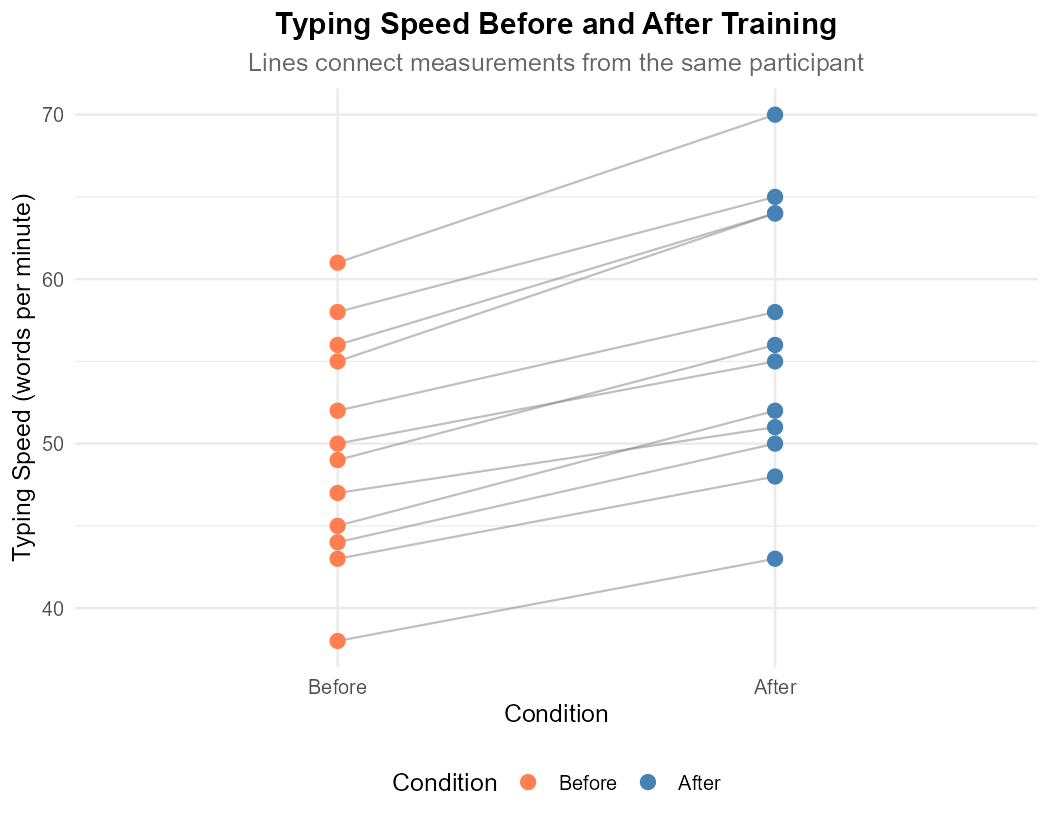
Fig. 11.7 Before-After measurements connected by subject

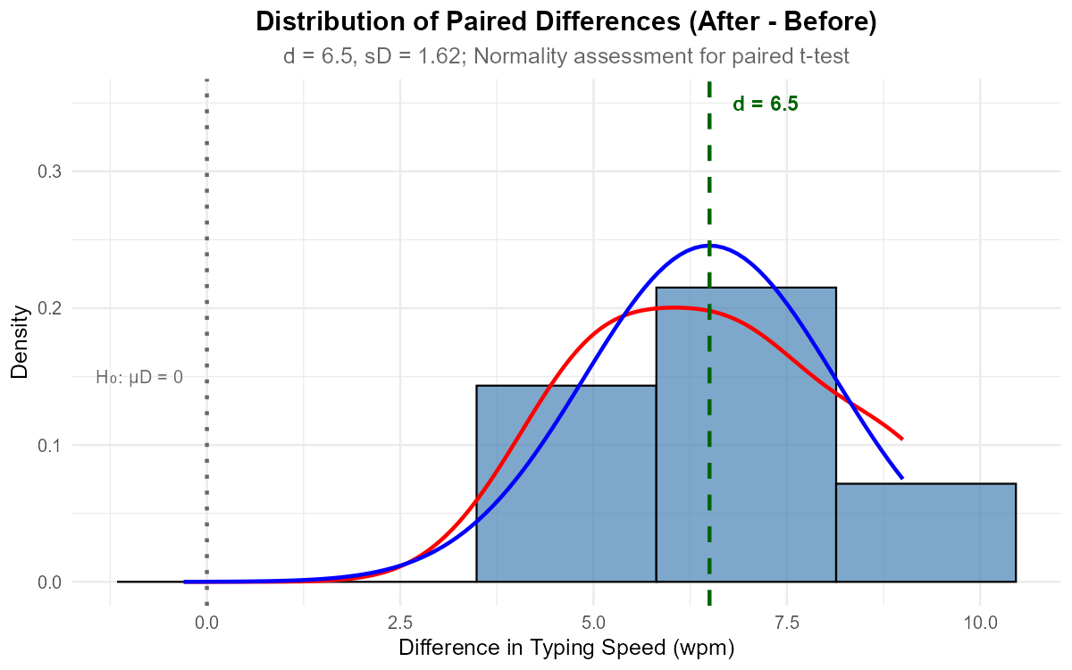
Fig. 11.8 Histogram of paired differences with normal overlay

1. Why is this a paired design rather than independent samples?

2. Calculate d̄ and s_D for the differences.

3. Using the histogram, assess whether the normality assumption for the differences is satisfied.

4. With n = 12, how important is the normality assumption? When would you be more concerned?

5. Conduct a paired t-test to determine if the training program improved typing speed at α = 0.05.

Solution

Part (a): Why paired?

This is a paired design because:

• Same subjects measured twice: Each participant provides both a “before” and “after” measurement

• Natural pairing: The measurements are linked by individual—participant 1’s before is paired with participant 1’s after

• Correlated measurements: A person who types fast before training will likely still type relatively fast after

Using independent samples would incorrectly ignore the within-subject correlation and likely have lower power.

Part (b): Summary statistics for differences

Differences D = After - Before: 7, 6, 5, 9, 4, 9, 5, 7, 5, 7, 6, 8

\[\bar{d} = \frac{7+6+5+9+4+9+5+7+5+7+6+8}{12} = \frac{78}{12} = 6.5\]

\[s_D = \sqrt{\frac{\sum(d_i - \bar{d})^2}{n-1}} = \sqrt{\frac{26}{11}} = 1.537\]

Part (c): Normality assessment from histogram

The histogram of differences shows:

• Approximately symmetric distribution

• Unimodal shape centered around 6-7

• No extreme outliers

• Kernel density and normal curve align reasonably well

Assessment: The normality assumption for differences appears satisfied ✓

Part (d): Importance of normality with n = 12

With n = 12, the normality assumption is moderately important because:

• Sample size is below the n ≥ 30 guideline for CLT

• The t-test is fairly robust to mild departures from normality

• Severe skewness or outliers would be concerning

We would be more concerned if:

• The histogram showed strong skewness

• There were extreme outliers in the differences

• The QQ-plot showed systematic curvature

• Sample size were even smaller (e.g., n < 8)

Part (e): Paired t-test

Step 1: Define the parameter

Let μ_D = true mean difference in typing speed (After - Before).

Step 2: State the hypotheses

Testing if training improves speed (positive difference):

\[H_0: \mu_D \leq 0 \quad \text{vs} \quad H_a: \mu_D > 0\]

Step 3: Check assumptions and calculate test statistic

Assumption checks:

• Paired design: Same subjects measured before and after ✓

• Independence of pairs: Participants are independent of each other ✓

• Normality of differences: Histogram supports approximate normality ✓

Test statistic:

\[t_{TS} = \frac{\bar{d} - 0}{s_D / \sqrt{n}} = \frac{6.5 - 0}{1.537 / \sqrt{12}} = \frac{6.5}{0.444} = 14.65\]

Degrees of freedom: df = n - 1 = 11

P-value (upper-tailed):

\[p\text{-value} = P(T_{11} > 14.65) < 0.0001\]

Step 4: Decision and Conclusion

Since p-value < 0.0001 < α = 0.05, reject H₀.

Conclusion: At the 0.05 significance level, there is overwhelming evidence that the ergonomic keyboard training program improves typing speed (p < 0.0001). The average improvement of 6.5 words per minute represents a meaningful gain for participants.

R verification:

before <- c(45, 52, 38, 61, 47, 55, 43, 58, 50, 49, 44, 56)
after <- c(52, 58, 43, 70, 51, 64, 48, 65, 55, 56, 50, 64)
d <- after - before

# Summary statistics
mean(d)  # 6.5
sd(d)    # 1.537

# Paired t-test
t.test(after, before, paired = TRUE, alternative = "greater")

# Or equivalently
t.test(d, mu = 0, alternative = "greater")

# Output: t = 14.65, df = 11, p-value < 0.0001

---

Exercise 6: Paired t-Test - Two-Tailed

A taste test compares two cola brands. Twelve participants rate each brand on a 1-100 scale:

Participant	Brand A	Brand B
1-4	72, 68, 81, 75	70, 65, 78, 72
5-8	69, 77, 73, 80	71, 74, 70, 76
9-12	74, 82, 70, 76	72, 79, 68, 75

1. Calculate the differences \(D = A - B\) and summary statistics.

2. Test whether there is a difference in mean ratings at α = 0.05.

3. Construct a 95% confidence interval for \(\mu_D\).

Solution

Part (a): Differences and summary statistics

Differences (A - B): 2, 3, 3, 3, -2, 3, 3, 4, 2, 3, 2, 1

\[\bar{d} = \frac{2+3+3+3+(-2)+3+3+4+2+3+2+1}{12} = \frac{27}{12} = 2.25\]

\[s_d = \sqrt{\frac{\sum(d_i - \bar{d})^2}{11}} = \sqrt{\frac{26.25}{11}} = \sqrt{2.386} = 1.545\]

Part (b): Hypothesis Test

Step 1: Let \(\mu_D\) = true mean difference in rating (Brand A - Brand B).

Step 2:

\[\begin{split}&H_0: \mu_D = 0\\ &H_a: \mu_D \neq 0\end{split}\]

Step 3:

\[SE = \frac{1.545}{\sqrt{12}} = 0.446\]

\[t_{TS} = \frac{2.25 - 0}{0.446} = 5.04\]

df = 11

P-value: \(2 \times P(T_{11} > 5.04) = 0.0004\)

Step 4: Since p = 0.0004 < 0.05, reject H₀.

The data does give strong support (p-value = 0.0004) to the claim that the mean ratings differ between the two cola brands. Brand A is rated higher on average.

Part (c): 95% Confidence Interval

Critical value: \(t_{0.025, 11} = 2.201\)

\[CI: 2.25 \pm 2.201 \times 0.446 = 2.25 \pm 0.98 = (1.27, 3.23)\]

We are 95% confident that Brand A is rated between 1.27 and 3.23 points higher than Brand B on average.

R verification:

A <- c(72, 68, 81, 75, 69, 77, 73, 80, 74, 82, 70, 76)
B <- c(70, 65, 78, 72, 71, 74, 70, 76, 72, 79, 68, 75)

t.test(A, B, paired = TRUE, alternative = "two.sided")
# t = 5.04, df = 11, p = 0.0004
# 95% CI: (1.27, 3.23)

---

Exercise 7: Paired t-Test - Lower-Tailed

A nursing sensitivity training program is evaluated. Eight nurses’ sensitivity scores are measured before and after training:

Summary statistics for \(D = \text{Before} - \text{After}\):

• \(n = 8\)

• \(\bar{d} = -1.30\)

• \(s_d = 0.86\)

Test whether the training improves sensitivity scores at α = 0.01.

Solution

Step 1: Define the parameter

Let \(\mu_D\) = true mean difference in sensitivity score (Before - After).

If training improves scores, then “After” > “Before”, so D = Before - After is negative.

Step 2: State the hypotheses

\[\begin{split}&H_0: \mu_D \geq 0\\ &H_a: \mu_D < 0\end{split}\]

Step 3: Calculate test statistic and p-value

\[SE = \frac{0.86}{\sqrt{8}} = \frac{0.86}{2.828} = 0.304\]

\[t_{TS} = \frac{-1.30 - 0}{0.304} = -4.28\]

df = 7

P-value (lower-tailed):

\[p = P(T_7 < -4.28) = 0.0018\]

Step 4: Decision and Conclusion

Since p = 0.0018 < α = 0.01, reject H₀.

The data does give strong support (p-value = 0.002) to the claim that the training program improves nurses’ sensitivity scores. The average improvement is 1.30 points.

R verification:

n <- 8; d_bar <- -1.30; s_d <- 0.86
SE <- s_d / sqrt(n)
t_ts <- d_bar / SE  # -4.28
pt(t_ts, df = 7, lower.tail = TRUE)  # 0.0018

---

Exercise 8: Confidence Bounds for Paired Data

A manufacturing process improvement is tested on 15 machines. Production rates (units/hour) are measured before and after the improvement.

For \(D = \text{After} - \text{Before}\):

• \(n = 15\)

• \(\bar{d} = 3.2\)

• \(s_d = 2.8\)

1. Construct a 95% confidence interval for \(\mu_D\).

2. Construct a 95% lower confidence bound for \(\mu_D\).

3. Interpret each confidence region in context.

4. Based on the LCB, can we conclude the improvement is at least 2 units/hour?

Solution

Preliminary calculations:

\[SE = \frac{2.8}{\sqrt{15}} = 0.723\]

df = 14

Part (a): 95% Confidence Interval

\(t_{0.025, 14} = 2.145\)

\[CI: 3.2 \pm 2.145 \times 0.723 = 3.2 \pm 1.55 = (1.65, 4.75)\]

Part (b): 95% Lower Confidence Bound

\(t_{0.05, 14} = 1.761\)

\[LCB = 3.2 - 1.761 \times 0.723 = 3.2 - 1.27 = 1.93\]

Part (c): Interpretations

CI: We are 95% confident that the true mean improvement in production rate is between 1.65 and 4.75 units/hour.

LCB: We are 95% confident that the true mean improvement is at least 1.93 units/hour.

Part (d): Can we conclude improvement ≥ 2?

The 95% LCB is 1.93 units/hour. Since 1.93 < 2, we cannot conclude with 95% confidence that the improvement is at least 2 units/hour.

However, it’s close—a slightly larger sample might push the LCB above 2.

R verification:

n <- 15; d_bar <- 3.2; s_d <- 2.8
SE <- s_d / sqrt(n)  # 0.723

# 95% CI
t_crit_2 <- qt(0.025, 14, lower.tail = FALSE)  # 2.145
c(d_bar - t_crit_2*SE, d_bar + t_crit_2*SE)  # (1.65, 4.75)

# 95% LCB
t_crit_1 <- qt(0.05, 14, lower.tail = FALSE)  # 1.761
d_bar - t_crit_1*SE  # 1.93

---

Exercise 9: Paired vs. Independent Analysis Comparison

A researcher incorrectly analyzes paired data as independent samples. Consider:

• 10 subjects, each measured twice (before/after)

• Before: \(\bar{x}_1 = 50\), \(s_1 = 8\)

• After: \(\bar{x}_2 = 45\), \(s_2 = 9\)

• Differences: \(\bar{d} = 5\), \(s_d = 3\)

1. Calculate the test statistic and p-value using the correct paired analysis.

2. Calculate the test statistic and p-value using the incorrect independent analysis (unpooled).

3. Compare the results. Why is the paired analysis more powerful here?

4. Under what conditions would the paired analysis NOT be more powerful?

Solution

Part (a): Correct paired analysis

\[SE_{paired} = \frac{s_d}{\sqrt{n}} = \frac{3}{\sqrt{10}} = 0.949\]

\[t_{paired} = \frac{5}{0.949} = 5.27\]

df = 9

P-value: \(2 \times P(T_9 > 5.27) = 0.0005\)

Part (b): Incorrect independent analysis

\[\widehat{SE}_{indep} = \sqrt{\frac{8^2}{10} + \frac{9^2}{10}} = \sqrt{6.4 + 8.1} = \sqrt{14.5} = 3.808\]

\[t_{indep} = \frac{5}{3.808} = 1.31\]

Welch df ≈ 17.6

P-value: \(2 \times P(T_{17.6} > 1.31) = 0.207\)

Part (c): Comparison

Analysis | SE | t-statistic | p-value |

|----------|—–|-------------|———| | Paired | 0.949 | 5.27 | 0.0005 | | Independent | 3.808 | 1.31 | 0.207 |

The paired analysis is dramatically more powerful because:

1. Smaller SE: \(s_d = 3\) is much smaller than the individual SDs (8 and 9)

2. This occurs because within-subject variation is controlled

3. The correlation between before/after is positive (subjects who score high before tend to score high after)

4. The paired design “removes” this shared variation

Part (d): When paired is NOT more powerful

Paired analysis may not be more powerful when:

• Correlation is zero or negative: If there’s no relationship between paired observations

• Degrees of freedom matter more: Paired has df = n-1 vs. approximately 2n-2 for independent

• The pairing is artificial: Arbitrary pairing of unrelated observations adds no benefit

• High carryover effects: If the first measurement affects the second, this creates bias

R verification:

# Paired
SE_paired <- 3 / sqrt(10)
t_paired <- 5 / SE_paired
2 * pt(t_paired, df = 9, lower.tail = FALSE)  # 0.0005

# Independent
SE_indep <- sqrt(64/10 + 81/10)
t_indep <- 5 / SE_indep
nu <- (6.4 + 8.1)^2 / ((6.4)^2/9 + (8.1)^2/9)  # ≈ 17.6
2 * pt(t_indep, df = nu, lower.tail = FALSE)  # 0.207

---

Exercise 10: Complete Paired Analysis

A physical therapist evaluates whether a new stretching protocol reduces chronic back pain. Eight patients rate their pain (0-10 scale) before and after 6 weeks of treatment:

Patient	Before	After
1	7.5	5.2
2	6.8	4.9
3	8.2	6.1
4	5.9	5.0
5	7.1	4.5
6	6.5	5.8
7	8.0	5.5
8	7.3	5.3

1. Calculate the differences and summary statistics.

2. Check assumptions for the paired t-test.

3. Test whether the stretching protocol reduces pain at α = 0.05.

4. Construct a 95% confidence interval for the mean pain reduction.

5. Interpret your results in clinical terms.

Solution

Part (a): Differences and summary statistics

Define \(D = \text{Before} - \text{After}\) (positive = improvement)

Differences: 2.3, 1.9, 2.1, 0.9, 2.6, 0.7, 2.5, 2.0

\[\bar{d} = \frac{2.3+1.9+2.1+0.9+2.6+0.7+2.5+2.0}{8} = \frac{15.0}{8} = 1.875\]

\[s_d = \sqrt{\frac{\sum(d_i - 1.875)^2}{7}} = \sqrt{\frac{3.495}{7}} = \sqrt{0.4993} = 0.707\]

Part (b): Assumptions check

1. Independence between pairs: ✓ Different patients

2. Random sample of pairs: Assume patients were randomly selected

3. Normality of differences: With n=8, need to verify. All differences are positive and similar in magnitude; no obvious outliers. The small sample is a concern, but data appears reasonably symmetric.

Part (c): Hypothesis Test

Step 1: Let \(\mu_D\) = true mean reduction in pain score (Before - After).

Step 2:

\[\begin{split}&H_0: \mu_D \leq 0\\ &H_a: \mu_D > 0\end{split}\]

Step 3:

\[SE = \frac{0.707}{\sqrt{8}} = 0.250\]

\[t_{TS} = \frac{1.875 - 0}{0.250} = 7.50\]

df = 7

P-value: \(P(T_7 > 7.50) < 0.0001\)

Step 4: Since p < 0.0001 < 0.05, reject H₀.

The data does give strong support (p-value < 0.0001) to the claim that the stretching protocol reduces chronic back pain.

Part (d): 95% Confidence Interval

\(t_{0.025, 7} = 2.365\)

\[CI: 1.875 \pm 2.365 \times 0.250 = 1.875 \pm 0.591 = (1.28, 2.47)\]

Part (e): Clinical interpretation

• Statistical: Strong evidence the protocol works (p < 0.0001)

• Effect magnitude: Average pain reduction of 1.875 points on a 0-10 scale

• Clinical significance: A nearly 2-point reduction is typically considered clinically meaningful for pain scales

• CI interpretation: We’re 95% confident the true mean reduction is between 1.28 and 2.47 points

• All patients improved: Every patient showed pain reduction, strengthening confidence in the result

• Limitations: Small sample (n=8), no control group, possible placebo effect

R verification:

before <- c(7.5, 6.8, 8.2, 5.9, 7.1, 6.5, 8.0, 7.3)
after <- c(5.2, 4.9, 6.1, 5.0, 4.5, 5.8, 5.5, 5.3)

t.test(before, after, paired = TRUE, alternative = "greater")
# t = 7.505, df = 7, p < 0.0001

t.test(before, after, paired = TRUE, alternative = "two.sided")
# 95% CI: (1.28, 2.47)

---

11.5.10. Additional Practice Problems

True/False Questions (1 point each)

1. In a paired design, the sample sizes must be equal.

   Ⓣ or Ⓕ

2. The paired t-test has degrees of freedom \(n_A + n_B - 2\).

   Ⓣ or Ⓕ

3. \(\bar{d}\) always equals \(\bar{x}_A - \bar{x}_B\) in paired designs.

   Ⓣ or Ⓕ

4. Paired designs control for individual/subject variability.

   Ⓣ or Ⓕ

5. The paired t-test is essentially a one-sample t-test on the differences.

   Ⓣ or Ⓕ

6. Before-and-after studies should always use paired analysis.

   Ⓣ or Ⓕ

Multiple Choice Questions (2 points each)

7. The standard error for a paired t-test is:

   Ⓐ \(s_d / n\)

   Ⓑ \(s_d / \sqrt{n}\)

   Ⓒ \(\sqrt{s^2_A/n_A + s^2_B/n_B}\)

   Ⓓ \(s_d \times \sqrt{n}\)

8. Degrees of freedom for a paired t-test with 15 pairs is:

   Ⓐ 28

   Ⓑ 15

   Ⓒ 14

   Ⓓ 29

9. Which scenario requires paired analysis?

   Ⓐ Comparing heights of fathers and unrelated sons

   Ⓑ Comparing test scores before and after training for the same students

   Ⓒ Comparing salaries of men and women in different companies

   Ⓓ Comparing reaction times of coffee drinkers and tea drinkers

10. When is a paired design more powerful than an independent design?

    Ⓐ When the correlation between pairs is negative

    Ⓑ When the correlation between pairs is positive

    Ⓒ When sample sizes are very different

    Ⓓ When variances are very different

11. In a paired analysis, the parameter \(\mu_D\) equals:

    Ⓐ \(\mu_A + \mu_B\)

    Ⓑ \(\mu_A - \mu_B\)

    Ⓒ \(\mu_A / \mu_B\)

    Ⓓ \((\mu_A + \mu_B) / 2\)

12. Using independent analysis on paired data typically:

    Ⓐ Increases power

    Ⓑ Decreases standard error

    Ⓒ Increases standard error and decreases power

    Ⓓ Has no effect on results

Answers to Practice Problems

True/False Answers:

1. True — Each observation in Group A is paired with exactly one in Group B.

2. False — Paired t-test has df = n - 1, where n is the number of pairs.

3. True — The mean of differences equals the difference of means.

4. True — By comparing within subjects, individual variation is eliminated.

5. True — We compute differences first, then perform a one-sample t-test on those differences.

6. True — When the same subjects are measured before and after, pairing is natural and appropriate.

Multiple Choice Answers:

7. Ⓑ — Standard error is \(s_d/\sqrt{n}\), just like a one-sample t-test.

8. Ⓒ — df = n - 1 = 15 - 1 = 14.

9. Ⓑ — Same students measured twice creates natural pairs.

10. Ⓑ — Positive correlation means within-subject variation is high, which pairing controls for.

11. Ⓑ — \(\mu_D = E[D_i] = E[X_{Ai} - X_{Bi}] = \mu_A - \mu_B\).

12. Ⓒ — Independent analysis ignores the pairing structure, leading to larger SE and lower power.