Slides 📊

Download Chapter 6 slides (PPTX)

6.5. Uniform Distribution

After exploring the mathematical elegance and complexity of the normal distribution, we now turn to perhaps the simplest of all continuous distributions: the uniform distribution.

Road Map 🧭

• Understand the uniform distribution as representing constant probability density over a fixed interval.

• Develop geometric intuition for probability as rectangular areas.

• Learn the mathematical formulation of uniform PDF and CDF, and explore the key properties.

6.5.1. The Essence of Uniform Randomness

A uniform distribution assigns equal probability density to every point within its support interval \([a, b]\) for some \(a < b\).

The Uniform PDF

A continuous random variable \(X\) is said to follow a uniform distribution on the interval \([a, b]\) if it has a probability density function of the following form:

\[\begin{split}f_X(x) = \begin{cases} \frac{1}{b-a} & \text{for } a \leq x \leq b \\ 0 & \text{elsewhere} \end{cases}\end{split}\]

We write \(X \sim \text{Uniform}(a,b)\) or sometimes \(X \sim U(a,b)\).

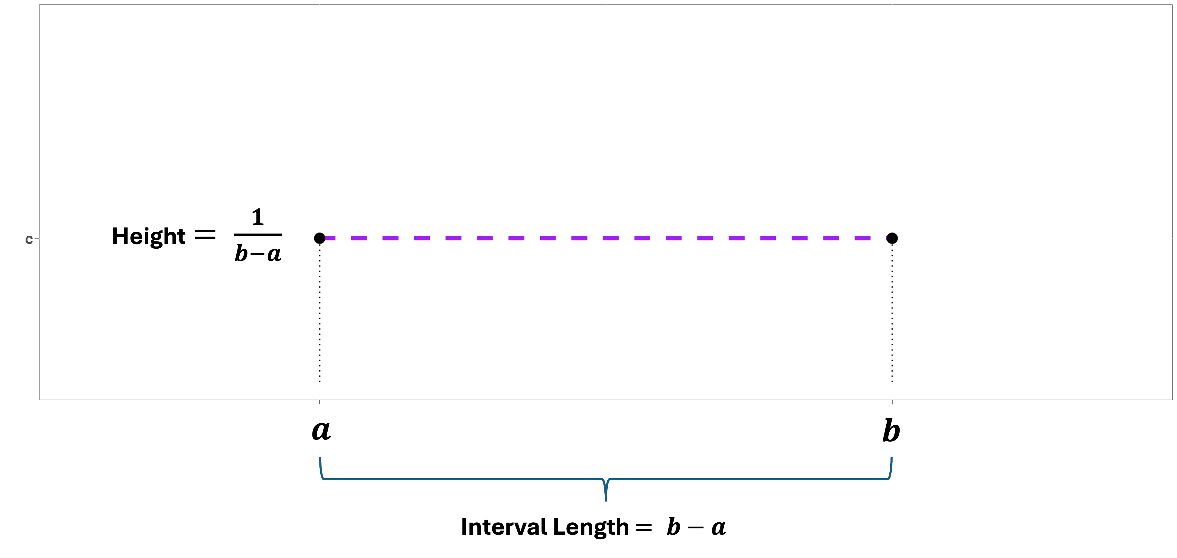
Fig. 6.47 A Uniform PDF

Determining the Constant Height

The constant \(\frac{1}{b-a}\) isn’t arbitrary—it’s the unique value that makes the PDF valid. Since the distribution forms a rectangle with base \((b-a)\) and height \(c\), the total area is \(\text{Area} = \text{base} \times \text{height} = (b-a) \times c\). For this to equal 1, we need:

\[(b-a) \times c = 1 \implies c = \frac{1}{b-a}\]

This geometric argument shows why the height must be the reciprocal of the interval length.

The Uniform CDF

The cumulative distribution function for a uniform distribution increases linearly from 0 to 1 over the support interval:

\[\begin{split}F_X(x) = \begin{cases} 0 & \text{for } x < a \\ \frac{x-a}{b-a} & \text{for } a \leq x < b \\ 1 & \text{for } x \geq b \end{cases}\end{split}\]

Fig. 6.48 A Uniform CDF

Deriving the CDF

• Before the rectangle begins, zero area is accummulated on the PDF. Thus the CDF is 0 for \(x < a\).

• After the rectangle is complete, all existing area in the PDF has been accummulated. The CDF is 1 for \(x \geq b\).

• For an \(x\) between \(a\) and \(b\), the CDF represents the size of the area under the PDF from \(-\infty\) to \(x\). Since the PDF is zero below \(a\) and constant at height \(\frac{1}{b-a}\) from \(a\) to \(x\), this region forms a rectangle with the width \(x-a\) and the height \(\frac{1}{b-a}\). Therefore,

\[F_X(x) = \text{width} \times \text{height} = (x-a) \times \frac{1}{b-a} = \frac{x-a}{b-a}.\]

6.5.2. The Length Principle

Since the uniform PDF has constant height \(\frac{1}{b-a}\) across its support, the probability of any interval equals the area of the corresponding rectangle:

\[\begin{split}P(c \leq X \leq d) &= \text{width} \times \text{height} = (d-c) \times \frac{1}{b-a} \\ &= \frac{d-c}{b-a} =\frac{\text{length of interval of interest}}{\text{total length of support}}\end{split}\]

Notice that this probability depends only on the interval length \((d-c)\) and the total support length \((b-a)\). The specific values of \(c\) and \(d\) don’t matter—only how far apart they are.

Example💡: Unifrom Probabilities

Consider \(X \sim \text{Uniform}(0, 10)\).

1. Find \(P(1 \leq X \leq 3)\).

   \[P(1 \leq X \leq 3) = \frac{3-1}{10-0} = \frac{2}{10} = 0.2\]

2. Find \(P(4.7 \leq X \leq 6.7)\).

   \[P(4.7 \leq X \leq 6.7) = \frac{6.7-4.7}{10-0} = \frac{2}{10} = 0.2\]

   Note that the two intervals in #1 and #2 have the same length. they also share the same probability.

3. Find \(P(8.5 \leq X \leq 10.5)\).

   \[\begin{split}P(8.5 \leq X \leq 10.5) &= P(8.5 \leq X \leq 10) + P(10 < X \leq 10.5)\\ &= \frac{1.5}{10} + 0 = 0.15\end{split}\]

   🛑 The interval in this probability statement extends beyond the support. Our calculation must reflect the fact that the probability of \(X\) taking any value greater than 10 is zero. This is an important example that highlights the role of the support in probability calculations.

6.5.3. Expected Value and Variance of Uniform Distribution

The uniform distribution’s symmetry and rectangular shape make its expected value geometrically obvious, while its variance can be computed through either geometric reasoning or algebraic integration.

Expected Value: The Midpoint

By symmetry, the expected value of a uniform random variable must lie at the center of its support:

\[E[X] = \mu_X = \frac{a+b}{2}\]

Algebraic Verification of Expected Value

We can confirm this geometric insight through integration:

\[\begin{split}E[X] &= \int_{-\infty}^{\infty} x \cdot f_X(x) \, dx = \int_a^b x \cdot \frac{1}{b-a} \, dx\\ &=\frac{1}{b-a} \int_a^b x \, dx = \frac{1}{b-a} \cdot \frac{x^2}{2}\Big|_a^b = \frac{1}{b-a} \cdot \frac{b^2-a^2}{2}\\ &= \frac{1}{b-a} \cdot \frac{(b-a)(b+a)}{2} = \frac{b+a}{2}✔\end{split}\]

Variance

For variance, we’ll use the computational formula \(\text{Var}(X) = E[X^2] - (E[X])^2\). We already know \(E[X]\), so we need to find \(E[X^2]\):

\[\begin{split}E[X^2] &= \int_a^b x^2 \cdot \frac{1}{b-a} \, dx = \frac{1}{b-a} \int_a^b x^2 \, dx\\ &= \frac{1}{b-a} \cdot \frac{x^3}{3}\Big|_a^b = \frac{1}{b-a} \cdot \frac{b^3-a^3}{3}\end{split}\]

Now we use the algebraic identity \(b^3 - a^3 = (b-a)(b^2 + ab + a^2)\):

\[E[X^2] = \frac{1}{b-a} \cdot \frac{(b-a)(b^2 + ab + a^2)}{3} = \frac{b^2 + ab + a^2}{3}\]

Finally, we compute the variance:

\[\begin{split}\text{Var}(X) &= E[X^2] - (E[X])^2 = \frac{b^2 + ab + a^2}{3} - \left(\frac{a+b}{2}\right)^2\\ &= \frac{b^2 + ab + a^2}{3} - \frac{a^2 + 2ab + b^2}{4}\\ &= \frac{4b^2 + 4ab + 4a^2 - 3a^2 - 6ab - 3b^2}{12}\\ &= \frac{b^2 - 2ab + a^2}{12} = \frac{(b-a)^2}{12}\end{split}\]

The Result

The variance and standard deviation of a uniform distribution is:

\[\text{Var}(X) = \frac{(b-a)^2}{12} \quad \text{ and } \quad \sigma_X = \sqrt{\text{Var}(X)} = \frac{b-a}{\sqrt{12}}\]

The variance depends only on the length of the support interval \((b-a)\)—wider intervals create more variability.

Example💡: Expectation, SD, and Percentile of a Uniform Random Variable

Suppose a factory produces metal bolts with diameters that fall between 10 mm and 30 mm evenly. Find the expected value, standard deviation, and the 25th percentile of the diameters.

Let \(X\) denote the diameters of metal bolts. \(X \sim \text{Uniform}(10, 30)\).

\[E[X] = \frac{10+30}{2} = 20\]

\[\sigma_x = \frac{30-10}{\sqrt{12}} = 5.7735\]

• For the 25th percentile \(x_{0.25}\), we must solve \(F_X(x_{0.25})=0.25\).

  \[\frac{x_{0.25}-a}{b-a} =0.25 \implies x_{0.25} = 10 + 0.25(30-10) = 10 + 5 = 15\]

  25% of the bolts produced in this factory has a diameter less than or equal to 15 mm.

6.5.4. Summary: Properties of Unifrom Distribution

• Notation: \(X \sim \text{Uniform}(a,b)\) or \(X \sim U(a,b)\)

• Parameters: \(a\) (lower bound) and \(b\) (upper bound), where \(a < b\)

• Support: \([a, b]\)

• PDF: \(f_X(x) = \begin{cases} \frac{1}{b-a} & \text{for } a \leq x \leq b \\ 0 & \text{elsewhere} \end{cases}\)

• CDF: \(F_X(x) = \begin{cases} 0 & \text{for } x < a \\ \frac{x-a}{b-a} & \text{for } a \leq x \leq b \\ 1 & \text{for } x > b \end{cases}\)

• Expected Value: \(E[X] = \frac{a+b}{2}\)

• Variance: \(\text{Var}(X) = \frac{(b-a)^2}{12}\)

• Standard Deviation: \(\sigma_X = \frac{b-a}{\sqrt{12}}\)

6.5.5. Bringing It All Together

Key Takeaways 📝

1. The uniform distribution represents constant probability density across a fixed interval, making it one of the simplest continuous distributions.

2. Only interval lengths matter for uniform probability calculations, as long as the interval is entirely inside the support.

3. The PDF height \(\frac{1}{b-a}\) ensures that the rectangular area equals 1.

4. The CDF increases linearly from 0 to 1 across the support.

5. Expected value equals the midpoint \(\frac{a+b}{2}\), and variance equals \(\frac{(b-a)^2}{12}\).

6.5.6. Exercises

These exercises develop your skills in working with uniform distributions, including computing probabilities using the length principle, finding expected values and variances, calculating percentiles, and handling cases where intervals extend beyond the support.

Key Formulas

For \(X \sim \text{Uniform}(a, b)\):

• PDF: \(f_X(x) = \frac{1}{b-a}\) for \(a \leq x \leq b\)

• CDF: \(F_X(x) = \frac{x-a}{b-a}\) for \(a \leq x \leq b\)

• Length Principle: \(P(c \leq X \leq d) = \frac{d-c}{b-a}\) (when \([c,d] \subseteq [a,b]\))

• General Probability Formula (handles intervals beyond support):

  \[P(c \leq X \leq d) = \frac{\text{length of } [c, d] \cap [a, b]}{b - a}\]

• Expected Value: \(E[X] = \frac{a+b}{2}\)

• Variance: \(\text{Var}(X) = \frac{(b-a)^2}{12}\)

Endpoint Note

For continuous distributions, \(P(X = c) = 0\) for any single point \(c\). Therefore, strict and non-strict inequalities yield the same probability: \(P(X < c) = P(X \leq c)\) and \(P(c < X < d) = P(c \leq X \leq d)\).

Exercise 1: Basic Uniform Properties

A network router distributes incoming data packets uniformly across a time window. The arrival time \(X\) (in milliseconds) of a randomly selected packet follows a \(\text{Uniform}(0, 50)\) distribution.

1. Write out the PDF \(f_X(x)\) for all regions of \(x\).

2. Find \(P(10 \leq X \leq 30)\).

3. Find \(P(X \leq 15)\).

4. Find \(P(X > 40)\).

5. Sketch the PDF and shade the region corresponding to part (b).

Solution

Let \(X\) = packet arrival time (ms), where \(X \sim \text{Uniform}(0, 50)\).

Part (a): PDF

The support is \([0, 50]\), so the height is \(\frac{1}{b-a} = \frac{1}{50-0} = \frac{1}{50} = 0.02\).

\[\begin{split}f_X(x) = \begin{cases} \frac{1}{50} = 0.02 & \text{for } 0 \leq x \leq 50 \\ 0 & \text{elsewhere} \end{cases}\end{split}\]

Part (b): P(10 ≤ X ≤ 30)

Using the length principle:

\[P(10 \leq X \leq 30) = \frac{30 - 10}{50 - 0} = \frac{20}{50} = 0.4\]

Part (c): P(X ≤ 15)

This is the CDF evaluated at 15:

\[P(X \leq 15) = F_X(15) = \frac{15 - 0}{50 - 0} = \frac{15}{50} = 0.3\]

Part (d): P(X > 40)

Using the complement:

\[P(X > 40) = 1 - P(X \leq 40) = 1 - \frac{40 - 0}{50 - 0} = 1 - 0.8 = 0.2\]

Part (e): Sketch

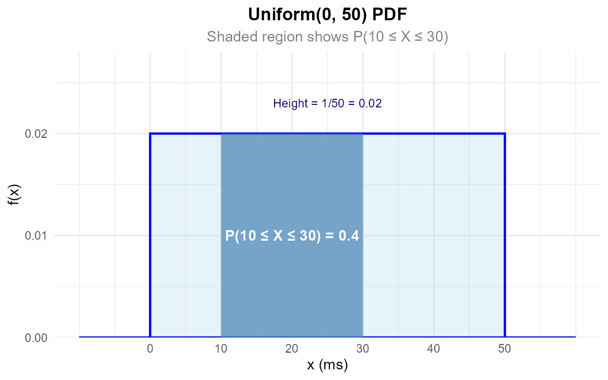
Fig. 6.49 The uniform PDF with P(10 ≤ X ≤ 30) = 0.4 shaded.

---

Exercise 2: Expected Value and Variance

A CNC milling machine produces cylindrical parts with diameters that follow a \(\text{Uniform}(24.8, 25.2)\) mm distribution due to inherent machine variability.

1. Find the expected diameter.

2. Find the variance and standard deviation of diameters.

3. A part is considered acceptable if its diameter is within 0.15 mm of the target (25.0 mm). What proportion of parts are acceptable?

4. Compare the standard deviation to the total range. What fraction of the range does one standard deviation represent?

Solution

Let \(X\) = part diameter (mm), where \(X \sim \text{Uniform}(24.8, 25.2)\).

Part (a): Expected value

\[E[X] = \frac{a + b}{2} = \frac{24.8 + 25.2}{2} = \frac{50.0}{2} = 25.0 \text{ mm}\]

The expected diameter equals the target—the machine is centered correctly.

Part (b): Variance and standard deviation

\[\text{Var}(X) = \frac{(b-a)^2}{12} = \frac{(25.2 - 24.8)^2}{12} = \frac{(0.4)^2}{12} = \frac{0.16}{12} = 0.01333 \text{ mm}^2\]

\[\sigma_X = \sqrt{0.01333} = 0.1155 \text{ mm}\]

Part (c): Proportion acceptable

Acceptable range: \(25.0 \pm 0.15 = [24.85, 25.15]\) mm.

\[P(24.85 \leq X \leq 25.15) = \frac{25.15 - 24.85}{25.2 - 24.8} = \frac{0.30}{0.40} = 0.75\]

75% of parts are acceptable.

Part (d): SD as fraction of range

Range = \(b - a = 0.4\) mm.

\[\frac{\sigma_X}{\text{Range}} = \frac{0.1155}{0.4} = 0.289 \approx \frac{1}{\sqrt{12}}\]

One standard deviation represents approximately 28.9% of the total range. This ratio \(\frac{1}{\sqrt{12}} \approx 0.289\) is a property of all uniform distributions.

---

Exercise 3: CDF Construction and Application

The voltage output of a sensor follows a \(\text{Uniform}(2.5, 4.5)\) V distribution.

1. Write out the CDF \(F_X(x)\) for all regions of \(x\).

2. Compute \(F_X(3.0)\), \(F_X(4.0)\), and \(F_X(5.0)\).

3. Use the CDF to find \(P(3.0 < X \leq 4.0)\).

4. Sketch the CDF and mark the values from part (b).

Solution

Let \(X\) = voltage output (V), where \(X \sim \text{Uniform}(2.5, 4.5)\).

Part (a): CDF for all regions

\[\begin{split}F_X(x) = \begin{cases} 0 & \text{for } x < 2.5 \\ \frac{x - 2.5}{4.5 - 2.5} = \frac{x - 2.5}{2} & \text{for } 2.5 \leq x \leq 4.5 \\ 1 & \text{for } x > 4.5 \end{cases}\end{split}\]

Part (b): CDF values

\[F_X(3.0) = \frac{3.0 - 2.5}{2} = \frac{0.5}{2} = 0.25\]

\[F_X(4.0) = \frac{4.0 - 2.5}{2} = \frac{1.5}{2} = 0.75\]

\[F_X(5.0) = 1 \quad \text{(since } 5.0 > 4.5 \text{)}\]

Part (c): P(3.0 < X ≤ 4.0)

\[P(3.0 < X \leq 4.0) = F_X(4.0) - F_X(3.0) = 0.75 - 0.25 = 0.50\]

Part (d): CDF sketch

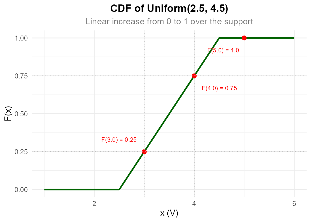
Fig. 6.50 The CDF increases linearly from 0 to 1 over the support [2.5, 4.5].

---

Exercise 4: Intervals Extending Beyond Support

A randomized algorithm selects a value uniformly from the interval \([5, 15]\). Let \(X\) denote this selected value.

1. Find \(P(8 \leq X \leq 12)\).

2. Find \(P(X \leq 3)\).

3. Find \(P(12 \leq X \leq 18)\).

4. Find \(P(X \geq 20)\).

5. Find \(P(2 \leq X \leq 22)\).

Solution

Let \(X \sim \text{Uniform}(5, 15)\).

Part (a): P(8 ≤ X ≤ 12) — interval entirely within support

\[P(8 \leq X \leq 12) = \frac{12 - 8}{15 - 5} = \frac{4}{10} = 0.4\]

Part (b): P(X ≤ 3) — entirely below support

Since \(3 < 5 = a\), no probability mass exists below 3.

\[P(X \leq 3) = 0\]

Part (c): P(12 ≤ X ≤ 18) — interval extends beyond upper bound

The support ends at 15, so we must truncate the interval:

\[P(12 \leq X \leq 18) = P(12 \leq X \leq 15) + P(15 < X \leq 18) = \frac{15 - 12}{10} + 0 = \frac{3}{10} = 0.3\]

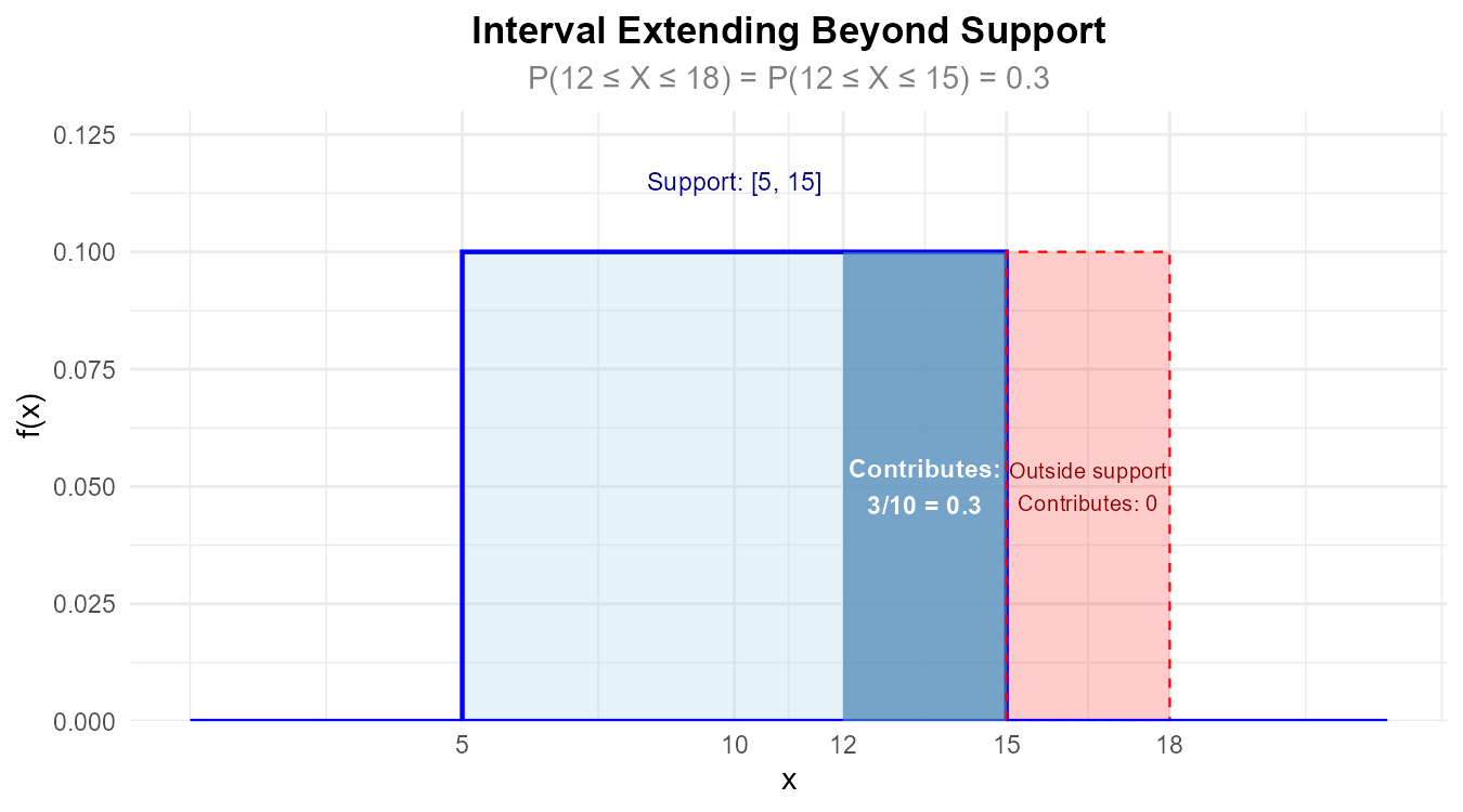
Fig. 6.51 Only the portion [12, 15] contributes to probability; the region [15, 18] is outside the support.

Part (d): P(X ≥ 20) — entirely above support

Since \(20 > 15 = b\), no probability mass exists above 15.

\[P(X \geq 20) = 0\]

Part (e): P(2 ≤ X ≤ 22) — interval contains entire support

The interval \([2, 22]\) completely contains the support \([5, 15]\).

\[P(2 \leq X \leq 22) = P(5 \leq X \leq 15) = \frac{15 - 5}{15 - 5} = 1\]

---

Exercise 5: Percentiles and Quartiles

The time (in minutes) for a 3D printer to complete a calibration cycle follows a \(\text{Uniform}(3, 7)\) distribution.

1. Find the median calibration time.

2. Find the first quartile \(Q_1\) (25th percentile).

3. Find the third quartile \(Q_3\) (75th percentile).

4. Calculate the interquartile range (IQR).

5. Find the 90th percentile of calibration times.

6. Verify that the IQR equals half the range for a uniform distribution.

Solution

Let \(X\) = calibration time (min), where \(X \sim \text{Uniform}(3, 7)\).

For the \(p\)-th percentile, solve \(F_X(x_p) = p\):

\[\frac{x_p - a}{b - a} = p \implies x_p = a + p(b - a)\]

Part (a): Median (50th percentile)

\[x_{0.50} = 3 + 0.50(7 - 3) = 3 + 2 = 5 \text{ min}\]

Note: The median equals the mean \(E[X] = \frac{3+7}{2} = 5\) for uniform distributions.

Part (b): First quartile Q₁ (25th percentile)

\[x_{0.25} = 3 + 0.25(7 - 3) = 3 + 1 = 4 \text{ min}\]

Part (c): Third quartile Q₃ (75th percentile)

\[x_{0.75} = 3 + 0.75(7 - 3) = 3 + 3 = 6 \text{ min}\]

Part (d): Interquartile range

\[\text{IQR} = Q_3 - Q_1 = 6 - 4 = 2 \text{ min}\]

Part (e): 90th percentile

\[x_{0.90} = 3 + 0.90(7 - 3) = 3 + 3.6 = 6.6 \text{ min}\]

Part (f): Verify IQR = Range/2

Range = \(b - a = 7 - 3 = 4\) min.

\[\frac{\text{Range}}{2} = \frac{4}{2} = 2 = \text{IQR} \quad \checkmark\]

This relationship holds for all uniform distributions since:

\[\text{IQR} = x_{0.75} - x_{0.25} = [a + 0.75(b-a)] - [a + 0.25(b-a)] = 0.5(b-a) = \frac{\text{Range}}{2}\]

---

Exercise 6: Comparing Probabilities

Two different measurement systems are used to record temperature. System A produces readings that follow \(\text{Uniform}(18, 26)\) °C, while System B produces readings that follow \(\text{Uniform}(20, 28)\) °C.

1. For each system, find the probability that a reading falls between 21 and 25 °C.

2. Find the expected value and standard deviation for each system.

3. Which system has more variability? Why?

4. What is the probability that a System A reading exceeds 26 °C? What about System B?

Solution

System A: \(X_A \sim \text{Uniform}(18, 26)\) with range = 8

System B: \(X_B \sim \text{Uniform}(20, 28)\) with range = 8

Part (a): P(21 ≤ X ≤ 25) for each system

System A: The interval [21, 25] is entirely within [18, 26].

\[P(21 \leq X_A \leq 25) = \frac{25 - 21}{26 - 18} = \frac{4}{8} = 0.5\]

System B: The interval [21, 25] is entirely within [20, 28].

\[P(21 \leq X_B \leq 25) = \frac{25 - 21}{28 - 20} = \frac{4}{8} = 0.5\]

Both probabilities are equal because both distributions have the same range (8), and the interval [21, 25] lies entirely within both supports. When an interval of interest is fully contained in the support, probability depends only on the ratio of interval length to range.

Note

This “same probability for same interval length” property holds only when the interval lies entirely within both supports. For example, P(17 ≤ X_A ≤ 21) ≠ P(17 ≤ X_B ≤ 21) because [17, 21] extends below System B’s support.

Part (b): Expected value and standard deviation

System A:

\[E[X_A] = \frac{18 + 26}{2} = 22 \text{ °C}\]

\[\sigma_A = \frac{26 - 18}{\sqrt{12}} = \frac{8}{\sqrt{12}} = 2.309 \text{ °C}\]

System B:

\[E[X_B] = \frac{20 + 28}{2} = 24 \text{ °C}\]

\[\sigma_B = \frac{28 - 20}{\sqrt{12}} = \frac{8}{\sqrt{12}} = 2.309 \text{ °C}\]

Part (c): Variability comparison

Both systems have equal variability (\(\sigma = 2.309\) °C) because they have the same range. The variance of a uniform distribution depends only on the range \((b-a)\), not on where the interval is located.

Part (d): P(X > 26) for each system

System A: Since 26 is the upper bound, \(P(X_A > 26) = 0\).

System B:

\[P(X_B > 26) = \frac{28 - 26}{28 - 20} = \frac{2}{8} = 0.25\]

---

Exercise 7: PDF Validity Check

Determine whether each of the following functions could be a valid PDF for a uniform distribution. If valid, identify the parameters \(a\) and \(b\). If not valid, explain why.

1. \(f(x) = 0.2\) for \(0 \leq x \leq 5\), and \(f(x) = 0\) elsewhere.

2. \(f(x) = 0.25\) for \(2 \leq x \leq 5\), and \(f(x) = 0\) elsewhere.

3. \(f(x) = \frac{1}{8}\) for \(-2 \leq x \leq 6\), and \(f(x) = 0\) elsewhere.

4. \(f(x) = -0.1\) for \(0 \leq x \leq 10\), and \(f(x) = 0\) elsewhere.

Solution

For a valid uniform PDF: (1) \(f(x) \geq 0\) for all \(x\), and (2) total area = 1.

Part (a): f(x) = 0.2 on [0, 5]

• Non-negativity: ✓ (0.2 > 0)

• Total area: \(0.2 \times 5 = 1\) ✓

Valid: \(\text{Uniform}(0, 5)\) with \(a = 0\), \(b = 5\).

Part (b): f(x) = 0.25 on [2, 5]

• Non-negativity: ✓ (0.25 > 0)

• Total area: \(0.25 \times (5 - 2) = 0.25 \times 3 = 0.75 \neq 1\) ✗

Not valid: The area under the curve is only 0.75, not 1. For Uniform(2, 5), the height should be \(\frac{1}{3} \approx 0.333\).

Part (c): f(x) = 1/8 on [-2, 6]

• Non-negativity: ✓ (1/8 > 0)

• Total area: \(\frac{1}{8} \times (6 - (-2)) = \frac{1}{8} \times 8 = 1\) ✓

Valid: \(\text{Uniform}(-2, 6)\) with \(a = -2\), \(b = 6\).

Part (d): f(x) = -0.1 on [0, 10]

• Non-negativity: ✗ (-0.1 < 0)

Not valid: A PDF cannot be negative. Probabilities (areas) must be non-negative.

---

Exercise 8: Reverse Engineering Parameters

A uniform random variable \(X\) has the following properties. Find the parameters \(a\) and \(b\) in each case.

1. \(E[X] = 10\) and \(\text{Var}(X) = 3\).

2. The median is 15 and the IQR is 6.

3. \(P(X \leq 8) = 0.4\) and \(P(X \leq 18) = 0.9\).

4. The PDF height is 0.05 and \(E[X] = 30\).

Solution

Part (a): E[X] = 10 and Var(X) = 3

From expected value: \(\frac{a+b}{2} = 10 \implies a + b = 20\)

From variance: \(\frac{(b-a)^2}{12} = 3 \implies (b-a)^2 = 36 \implies b - a = 6\)

Solving the system:

• \(a + b = 20\)

• \(b - a = 6\)

Adding: \(2b = 26 \implies b = 13\)

Subtracting: \(2a = 14 \implies a = 7\)

Answer: \(a = 7\), \(b = 13\).

Part (b): Median = 15 and IQR = 6

For uniform distributions, median = mean = \(\frac{a+b}{2} = 15 \implies a + b = 30\).

IQR = \(\frac{b-a}{2} = 6 \implies b - a = 12\).

Solving:

• Adding: \(2b = 42 \implies b = 21\)

• Subtracting: \(2a = 18 \implies a = 9\)

Answer: \(a = 9\), \(b = 21\).

Part (c): P(X ≤ 8) = 0.4 and P(X ≤ 18) = 0.9

Both values are interior CDF values, so both 8 and 18 are within the support \([a, b]\).

Using the CDF formula \(F_X(x) = \frac{x - a}{b - a}\):

\[\frac{8 - a}{b - a} = 0.4 \implies 8 - a = 0.4(b - a)\]

\[\frac{18 - a}{b - a} = 0.9 \implies 18 - a = 0.9(b - a)\]

Dividing the second equation by the first:

\[\frac{18 - a}{8 - a} = \frac{0.9}{0.4} = 2.25\]

Cross-multiplying: \(18 - a = 2.25(8 - a) = 18 - 2.25a\)

Solving: \(-a + 2.25a = 0 \implies 1.25a = 0 \implies a = 0\)

Substituting \(a = 0\) into the first equation:

\(8 = 0.4b \implies b = 20\)

Verification: \(F_X(8) = \frac{8}{20} = 0.4\) ✓ and \(F_X(18) = \frac{18}{20} = 0.9\) ✓

Answer: \(a = 0\), \(b = 20\).

Part (d): PDF height = 0.05 and E[X] = 30

From PDF height: \(\frac{1}{b-a} = 0.05 \implies b - a = 20\)

From expected value: \(\frac{a+b}{2} = 30 \implies a + b = 60\)

Solving:

• Adding: \(2b = 80 \implies b = 40\)

• Subtracting: \(2a = 40 \implies a = 20\)

Answer: \(a = 20\), \(b = 40\).

---

Exercise 9: Application — Quality Control

A filling machine dispenses liquid into containers. The amount dispensed (in mL) follows a \(\text{Uniform}(495, 505)\) distribution.

1. Find the expected amount and standard deviation of liquid dispensed.

2. Quality specifications require containers to have between 497 and 503 mL. What proportion of containers meet specifications?

3. A container is rejected as “underfilled” if it contains less than 496 mL. What proportion is rejected?

4. Management wants to adjust the machine so that at most 5% of containers are underfilled (< 496 mL). If the range stays at 10 mL, what should the new lower bound \(a\) be?

5. After the adjustment in part (d), what proportion of containers will have more than 504 mL?

Solution

Current machine: \(X \sim \text{Uniform}(495, 505)\).

Part (a): Expected value and standard deviation

\[E[X] = \frac{495 + 505}{2} = 500 \text{ mL}\]

\[\sigma_X = \frac{505 - 495}{\sqrt{12}} = \frac{10}{\sqrt{12}} = 2.887 \text{ mL}\]

Part (b): Proportion meeting specs [497, 503]

\[P(497 \leq X \leq 503) = \frac{503 - 497}{505 - 495} = \frac{6}{10} = 0.60\]

60% of containers meet specifications.

Part (c): Proportion underfilled (< 496 mL)

\[P(X < 496) = \frac{496 - 495}{505 - 495} = \frac{1}{10} = 0.10\]

10% of containers are rejected as underfilled.

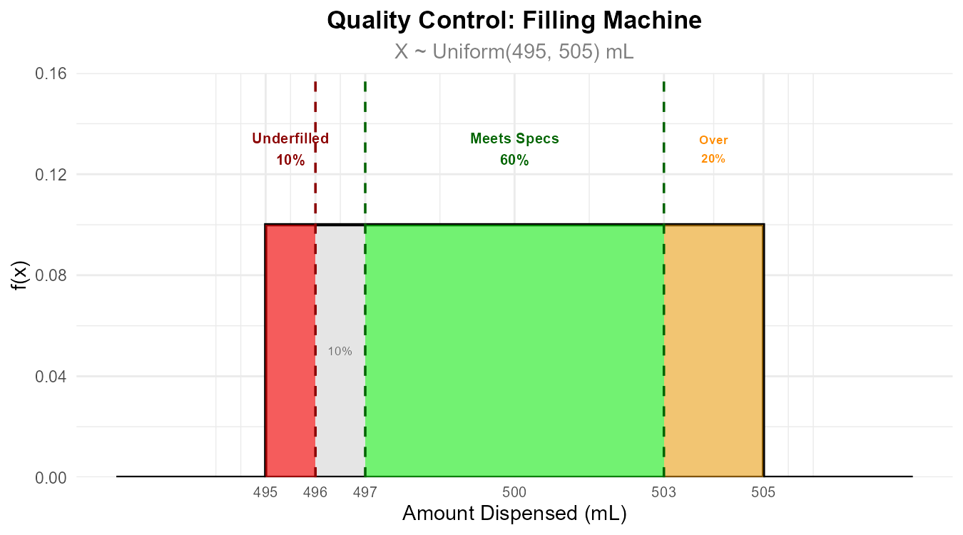
Fig. 6.52 Current machine: 10% underfilled, 60% meeting specs.

Part (d): Adjust to have at most 5% underfilled

We need \(P(X < 496) \leq 0.05\) with range = 10 (so \(b = a + 10\)).

For exactly 5% underfilled:

\[\frac{496 - a}{(a+10) - a} = 0.05 \implies \frac{496 - a}{10} = 0.05\]

\[496 - a = 0.5 \implies a = 495.5\]

So the new distribution is \(\text{Uniform}(495.5, 505.5)\).

Answer: \(a = 495.5\) mL (shift the distribution up by 0.5 mL).

Part (e): Proportion > 504 mL after adjustment

With \(X \sim \text{Uniform}(495.5, 505.5)\):

\[P(X > 504) = \frac{505.5 - 504}{505.5 - 495.5} = \frac{1.5}{10} = 0.15\]

15% of containers will have more than 504 mL.

---

6.5.7. Additional Practice Problems

True/False Questions (1 point each)

1. For a uniform distribution, the expected value always equals the median.

   Ⓣ or Ⓕ

2. If \(X \sim \text{Uniform}(0, 10)\), then \(P(2 \leq X \leq 4) = P(7 \leq X \leq 9)\).

   Ⓣ or Ⓕ

3. The variance of \(\text{Uniform}(a, b)\) depends on both \(a\) and \(b\) individually, not just their difference.

   Ⓣ or Ⓕ

4. For \(X \sim \text{Uniform}(5, 15)\), \(P(X = 10) = 0.1\).

   Ⓣ or Ⓕ

5. The CDF of a uniform distribution is a straight line throughout its entire domain.

   Ⓣ or Ⓕ

6. If \(X \sim \text{Uniform}(0, 20)\), then \(P(X > 25) = 0\).

   Ⓣ or Ⓕ

7. The IQR of any uniform distribution equals half of its range.

   Ⓣ or Ⓕ

8. For \(X \sim \text{Uniform}(a, b)\), the PDF height \(\frac{1}{b-a}\) can be greater than 1.

   Ⓣ or Ⓕ

Multiple Choice Questions (2 points each)

9. For \(X \sim \text{Uniform}(10, 30)\), what is \(E[X]\)?

   Ⓐ 10

   Ⓑ 15

   Ⓒ 20

   Ⓓ 30

10. For \(X \sim \text{Uniform}(0, 6)\), what is \(\text{Var}(X)\)?

    Ⓐ 0.5

    Ⓑ 1

    Ⓒ 3

    Ⓓ 6

11. For \(X \sim \text{Uniform}(4, 12)\), what is \(P(6 \leq X \leq 10)\)?

    Ⓐ 0.25

    Ⓑ 0.4

    Ⓒ 0.5

    Ⓓ 0.75

12. For \(X \sim \text{Uniform}(0, 8)\), what is the 75th percentile?

    Ⓐ 2

    Ⓑ 4

    Ⓒ 6

    Ⓓ 8

13. For \(X \sim \text{Uniform}(5, 25)\), what is \(P(0 \leq X \leq 10)\)?

    Ⓐ 0

    Ⓑ 0.25

    Ⓒ 0.5

    Ⓓ 1

14. Which of the following is a valid uniform PDF?

    Ⓐ \(f(x) = 0.5\) for \(0 \leq x \leq 4\)

    Ⓑ \(f(x) = 0.1\) for \(0 \leq x \leq 10\)

    Ⓒ \(f(x) = 0.2\) for \(0 \leq x \leq 4\)

    Ⓓ \(f(x) = 2\) for \(0 \leq x \leq 1\)

Answers to Practice Problems

True/False Answers:

1. True — For uniform distributions, mean = median = \(\frac{a+b}{2}\) due to perfect symmetry.

2. True — Both intervals have length 2, and for uniform distributions, \(P(c \leq X \leq d)\) depends only on interval length when the interval is within the support.

3. False — The variance formula \(\frac{(b-a)^2}{12}\) depends only on the range \((b-a)\), not on \(a\) and \(b\) individually.

4. False — For continuous distributions, \(P(X = c) = 0\) for any single point \(c\).

5. False — The CDF is a straight line only over the support \([a, b]\). It equals 0 for \(x < a\) and 1 for \(x > b\).

6. True — The support is \([0, 20]\), so no probability exists above 20.

7. True — \(\text{IQR} = x_{0.75} - x_{0.25} = 0.75(b-a) - 0.25(b-a) = 0.5(b-a) = \frac{\text{Range}}{2}\).

8. True — If \(b - a < 1\), then \(\frac{1}{b-a} > 1\). For example, Uniform(0, 0.5) has PDF height 2.

Multiple Choice Answers:

9. Ⓒ — \(E[X] = \frac{10 + 30}{2} = 20\).

10. Ⓒ — \(\text{Var}(X) = \frac{(6-0)^2}{12} = \frac{36}{12} = 3\).

11. Ⓒ — \(P(6 \leq X \leq 10) = \frac{10-6}{12-4} = \frac{4}{8} = 0.5\).

12. Ⓒ — \(x_{0.75} = 0 + 0.75(8-0) = 6\).

13. Ⓑ — The interval \([0, 10]\) overlaps with \([5, 25]\) only on \([5, 10]\). So \(P(0 \leq X \leq 10) = P(5 \leq X \leq 10) = \frac{10-5}{25-5} = \frac{5}{20} = 0.25\).

14. Ⓑ — Check each by computing area = height × width:

    • Ⓐ: \(0.5 \times 4 = 2 \neq 1\) ✗

    • Ⓑ: \(0.1 \times 10 = 1\) ✓

    • Ⓒ: \(0.2 \times 4 = 0.8 \neq 1\) ✗

    • Ⓓ: \(2 \times 1 = 2 \neq 1\) ✗