Slides 📊

Download Chapter 5 slides (PPTX)

5.1. Discrete Random Variables and Probability Mass Distributions

In previous chapters, we used set theory to describe events and their probabilities. While this approach provides a rigorous foundation, it can become cumbersome when dealing with complex scenarios. Random variables offer a more elegant solution by mapping outcomes directly to numbers.

Road Map 🧭

• Define random variables as functions that map real-life events of arbitrary complexity to their numerical representations.

• Distinguish between discrete and continuous random variables.

• Formalize probability mass functions (PMFs) for discrete random variables.

• Apply PMFs to calculate probabilities for complex events.

5.1.1. Random Variables: From Sets to Numbers

Definition

A random variable (RV) \(X\) is a function that maps each outcome in the sample space \(\omega \in \Omega\) to a numerical value. Formally, \(X: \Omega \to \mathbb{R}\).

Why is a Random Variable Needed?

Outcomes of random experiments are often multi-faceted and tend to introduce more complexity than necessary. For example, suppose we flip a coin 10 times and count how many heads appear in the sequence. The complete sample space of ten coin flips contains \(2^{10} = 1,024\) different possible sequences.

However, if we’re only interested in the total number of heads, we do not need to examine each sequence individually. For instance, instead of interpreting ‘HHHHHHHHTH’ as a unique sequence, we can view it simply as an outcome that yields the numerical value 9.

This is where a random variable becomes useful. We can define a random variable, say \(X\), to map the outcome ‘HHHHHHHHTH’ to a numerical value that reflects the focus of our interest:

\[X('HHHHHHHHTH') = 9,\]

and all other 1,023 outcomes in a similar manner. By using a random variable, we reduced our focus from 1,024 sequences to just 11 possible values (0 through 10).

Expressing Events With Random Variables

One of the key advantages of introducing a random variable is conciseness. Once an appropriate random variable is defined, most events can be expressed as equalities or inequalities involving the variable. See the table below for some examples:

Description	Using set notation	Using random variable \(X\)
Event that there are three heads in the sequence	Define \(A_3\) as the name of the event. List all sequences with three heads in \(A_3 = \{\cdots\}\).	\(X=3\)
Event that there are more than 7 heads in the sequence	Define \(A_8, A_9, A_{10}\) as the events of sequences with 8, 9, and 10 heads, respectively. The event of interest is \(A_8 \cup A_9 \cup A_{10}\).	\(X > 7\)

We no longer need to define a new event for every new question. Instead, we can express various situations compactly using the random variable \(X\).

5.1.2. Types of Random Variables

Random variables fall into two main categories based on the nature of their possible values.

Discrete Random Variables

A random variable is discrete if it can take on only a countable number of possible values. Discrete random variables typically arise when counting things, such as:

• The number of heads in coin flips

• The number of website hits during a specific time period

• The number of customers until the first big-ticket item is sold

Continuous Random Variables

A random variable is continuous if it can take on any value within a continuous range or interval. Continuous random variables typically arise when measuring quantities, such as:

• Height, weight, or other physical measurements

• Time until a particular event occurs

• Temperature, pressure, or other environmental measurements

5.1.3. Probability Distributions

To describe the probabilistic behavior of a random variable, we must specify the probabilities associated with all its possible values. This complete description is called a probability distribution.

Discrete and continuous random variables have different types of probability distributions. Discrete random variables is described by a probability mass function (PMF), while a continuous random variables is described by a probability density function (PDF).

In this chapter, we will focus on discrete random variables and PMFs. As we progress through the course, we will see how PMFs and PDFs share some foundational ideas, while differing in important ways.

5.1.4. Probability Mass Functions

Definition

The probability mass function of a discrete random variable \(X\) is denoted by \(p_X\). For each possible value \(x\) that \(X\) can take, it gives

\[p_X(x) = P(X = x).\]

Different forms of a PMF

A PMF can be represented in several different forms.

1. A PMF can be organized into a table by listing the possible values with their corresponding probabilities.

   

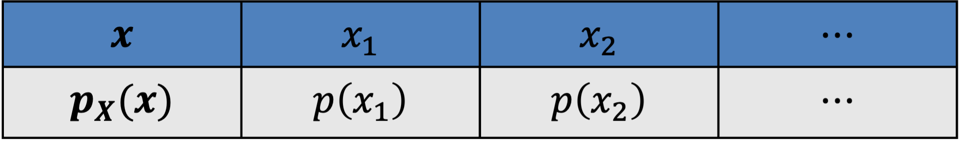
   Fig. 5.1 Exapmle of a PMF in table form

2. A bar graph can visually represent a PMF, with possible values on the x-axis and bar heights indicating their probabilities. However, it is rarely used alone, since exact probabilities are hard to read unless the plot is very simple.

3. For some special random variables, a mathematical formula is used to describe the PMF. One example is:

   \[p_X(x) = \frac{e^{-\lambda} \lambda^x}{x!}, \text{ for } x \geq 0\]

Support

The support of a discrete random variable is the set of all possible values with a positive probability:

\[\text{supp}(X) = \{x \in \mathbb{R} \mid p_X(x) > 0\}.\]

Validity of a PMF

For a probability mass function to be valid, the following conditions must hold.

1. Non-negativity: For all \(x\), \(0 \leq p_X(x) \leq 1.\)

2. Total probability of 1: The sum of probabilities over all values in the support must equal 1:

   \[\sum_{x \in \text{supp}(X)} p_X(x) = 1\]

5.1.5. Important Types of Problems Involving PMFs

A. Constructing a PMF from Scracth

It is an important skill for statisticians to be able to “translate” descriptions of a random experiment in plain language to mathematical language involving a random variable and its PMF.

Example💡: Flipping a Biased Coin

Let us try constructing a PMF from scratch, only using descriptions of the experimental setting.

Suppose we flip a biased coin four times, where the probability of heads on each flip is 0.7 (and tails is 0.3). We define a random variable \(H\) to count the number of heads in the four flips. Find the complete PMF for \(H\). Verify that the PMF is valid.

First, let’s identify the sample space. There are \(2^4 = 16\) possible sequences of heads and tails over four flips. However, rather than working with all 16 sequences individually, we can group them based on the number of heads:

• \(H = 0\): Only one sequence has zero heads (all tails: TTTT)

• \(H = 1\): Four sequences have exactly one head (HTTT, THTT, TTHT, TTTH)

• \(H = 2\): Six sequences have exactly two heads

• \(H = 3\): Four sequences have exactly three heads

• \(H = 4\): Only one sequence has all four heads (HHHH)

Using the independence of the coin flips and the given probabilities,

• \(P(H = 0) = P(TTTT) = (0.3)^4 = 0.0081\)

• \(P(H = 1) = 4 (0.3)^3 (0.7) = 0.0756\)

• \(P(H = 2) = 6 (0.3)^2 (0.7)^2 = 0.2646\)

• \(P(H = 3) = 4 (0.3) (0.7)^3 = 0.4116\)

• \(P(H = 4) = (0.7)^4 = 0.2401\)

All probabilities are betwen 0 and 1, satisfying the first condition for validity. The probabilities also sum to 1:

\[0.0081 + 0.0756 + 0.2646 + 0.4116 + 0.2401 = 1.\]

This gives us the complete PMF for our random variable \(H\).

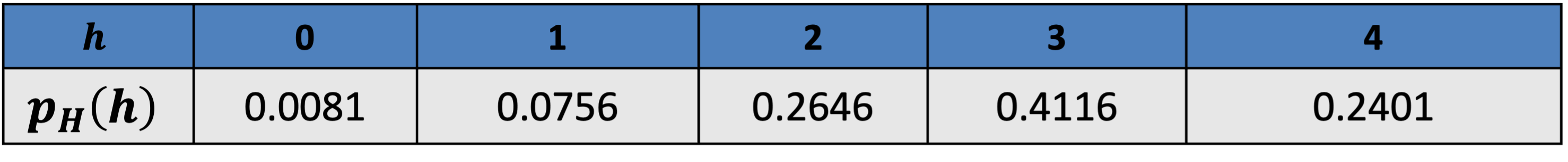
Fig. 5.2 Probability mass function for the number of heads in four flips

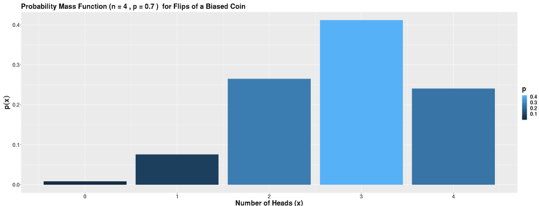
Fig. 5.3 Visualization of the PMF for the number of heads in four flips

The PMF reveals that getting three heads is the most likely outcome, with a probability of approximately 0.41, while getting zero heads is very unlikely, with a probability of only about 0.008.

B. Completing a Partially Known PMF

Completing a partially specified PMF is a common task in statistics. Typical scenarios include:

• One probability in the support is unknown.

• Multiple probabilities are unknown, with additional constraints provided.

• The coefficient \(k\) that turns a non-negative function \(f(x)\) into a valid PMF \(p_X(x) = kf(x)\) is unknown. This constant \(k\) is called the normalization constant.

In all cases, we must “fill in the blanks” by applying the conditions of a valid PMF.

Example💡: Finding the Normalization Constant

Consider a potential PMF:

\[\begin{split}p_X(x) = \begin{cases} \frac{k}{16} & \text{for } x = 0, 1 \\ \frac{k}{32} & \text{for } x = 2, 3, 4 \\ \frac{k}{64} & \text{for } x = 5, 6\\ 0 & \text{for all other} x \end{cases}\end{split}\]

To make this a valid PMF, we need to find the value of k that ensures the probabilities sum to 1:

\[\frac{k}{16} + \frac{k}{16} + \frac{k}{32} + \frac{k}{32} + \frac{k}{32} + \frac{k}{64} + \frac{k}{64} = 1\]

Multiplying both sides by 64 and solving for \(k\),

\[\begin{split}&4k + 4k + 2k + 2k + 2k + k + k = 64\\ &16k = 64 \\ &k = 4\end{split}\]

Therefore, the valid PMF is:

\[\begin{split}p_X(x) = \begin{cases} \frac{1}{4} & \text{for } x = 0, 1 \\ \frac{1}{8} & \text{for } x = 2, 3, 4 \\ \frac{1}{16} & \text{for } x = 5, 6\\ 0 & \text{for all other} x \end{cases}\end{split}\]

C. Calculating Probabilities with PMFs

Once we have a complete PMF, we can calculate probabilities for various events related to the random variable.

Viewing events as equalities and inequalities involving a random variable, we can express probablities of unions, intersections, and complements concisely in terms of \(p_X(x)\). Let us first get some practice writing proability statements correctly in terms of \(X\).

Example: Consider a random variable \(X\) whose support consists of all positive integers.

Probability statements for discrete RV \(X\) with a positive support
Description	Expresssion in terms of \(p_X(x)\)	Comment
Probability that X is less than 4	\[\begin{split}&P(X < 4) \\ &= P(X=1 \text{ OR } X=2 \text{ OR } X=3) \\ &= P(X=1 \cup X=2 \cup X=3)\\ &= P(X=1) + P(X=2) + P(X=3)\\ &= p_X(1) + p_X(2) + p_X(3)\end{split}\]	The transition from the third to the fourth line works because the events \(\{X=x\}\) are disjoint for different values of \(x\) (See the special addition rule).
Probability that X is less than 4 and at least 2	\[\begin{split}&P(X < 4 \cap X \geq 2)\\ &= P(2 \leq X < 4)\\ & = p_X(2) + p_X(3)\end{split}\]	For intersections and unions of non-disjoint events, think of ways to combine the two separate (in)equalities into one.
Probability that X is at least than 4 or greater than 6	\[\begin{split}&P(X4 \geq \cup X>6) \\ &= P(X \geq 4) \\ &= 1 - P(X < 4)\end{split}\]	To compute \(P(X \geq 4)\) directly, we would have to sum infinitely many terms. The complement rule simplifies computation.

Now, let us apply these skills to solve a problem.

Example💡: Computing probabilities using PMF

Using the PMF we just derived, let’s calculate some probabilities.

\[\begin{split}p_X(x) = \begin{cases} \frac{1}{4} & \text{for } x = 0, 1 \\ \frac{1}{8} & \text{for } x = 2, 3, 4 \\ \frac{1}{16} & \text{for } x = 5, 6\\ 0 & \text{for all other} x \end{cases}\end{split}\]

1. The probability that X is even:

   \[\begin{split}P(X \text{ is even}) &= P(X = 0) + P(X = 2) + P(X = 4) + P(X = 6) \\ &= 1/4 + 1/8 + 1/8 + 1/16 = 9/16\end{split}\]

2. The probability that X is greater than 3:

   \[\begin{split}P(X > 3) &= P(X = 4) + P(X = 5) + P(X = 6) \\ &= 1/8 + 1/16 + 1/16 = 1/4\end{split}\]

3. Are the events \(\{X = 5 or X = 6\}\) and \(\{X > 3\}\) independent?

   To show independence between two events \(A\) and \(B\), we must show that they meet the mathematical definition of idependence. That is, we must verify \(P(A|B) = P(A)\) or \(P(B|A)P(A).\)

   \[\begin{split}P(X = 5 \text{ or } X = 6 | X > 3) &= \frac{P((X = 5 \cup X = 6) \cap (X > 3))}{P(X > 3)}\\ &= \frac{P(X = 5 \cup X = 6)}{P(X > 3)}\\ &= (1/16 + 1/16)/(1/4) = 1/2\\ P(X = 5 \cup X = 6) &= 1/16 + 1/16 = 1/8\end{split}\]

   Since \(1/2 \neq 1/8\), these events are not independent.

5.1.6. Bringing It All Together

Key Takeaways 📝

1. Random variables map outcomes from the sample space to numerical values, allowing us to focus on quantities of interest rather than complex sets.

2. Discrete random variables take on countable values and are typically used when counting things, while continuous random variables can take any value in a continuum and are used for measurements.

3. A probability mass function (PMF) specifies the probability that a discrete random variable equals each possible value in its support.

4. Valid PMFs must satisfy two conditions:

   1. all probabilities are between 0 and 1, and

   2. the sum of all probabilities equals 1.

5. We can calculate probabilities for various events by rewriting the probability statements in terms of the PMF.

5.1.7. Exercises

These exercises develop your skills in defining random variables, constructing and validating PMFs, and calculating probabilities using PMFs.

Exercise 1: Defining Random Variables

For each scenario below, define an appropriate random variable and classify it as discrete or continuous. Identify the support (set of possible values) for each.

1. A quality control engineer inspects a batch of 8 circuit boards and counts how many have defects.

2. A data center monitors the time (in hours) until a server experiences its first hardware failure after being powered on.

3. A network security system tracks the number of failed login attempts to a server during a one-hour period.

4. A biomedical engineer measures the blood pressure (in mmHg) of patients during a clinical trial.

5. A software team releases an app update and tracks how many users out of the first 100 downloaders report bugs.

Solution

Part (a): Circuit Board Defects

• Random variable: Let \(X\) = number of defective circuit boards in the batch

• Type: Discrete (counting)

• Support: \(\text{supp}(X) = \{0, 1, 2, 3, 4, 5, 6, 7, 8\}\)

Part (b): Server Failure Time

• Random variable: Let \(T\) = time (in hours) until first hardware failure

• Type: Continuous (measuring time)

• Support: \(\text{supp}(T) = (0, \infty)\) or \([0, \infty)\) depending on interpretation

Part (c): Failed Login Attempts

• Random variable: Let \(N\) = number of failed login attempts in one hour

• Type: Discrete (counting)

• Support: \(\text{supp}(N) = \{0, 1, 2, 3, \ldots\}\) (non-negative integers)

Part (d): Blood Pressure

• Random variable: Let \(B\) = blood pressure measurement (mmHg)

• Type: Continuous (measuring)

• Support: \(\text{supp}(B) = (0, \infty)\) in theory, or a practical range like \([60, 200]\)

Part (e): Bug Reports

• Random variable: Let \(R\) = number of users (out of 100) who report bugs

• Type: Discrete (counting)

• Support: \(\text{supp}(R) = \{0, 1, 2, \ldots, 100\}\)

Key Distinction: Discrete random variables arise from counting (how many), while continuous random variables arise from measuring (how much/long/far).

---

Exercise 2: Constructing a PMF from Scratch

A software testing process involves running 3 independent test cases on a new feature. Each test case has a 70% probability of passing (and 30% probability of failing) independently.

Let \(X\) = the number of test cases that pass.

1. What is the support of \(X\)?

2. List all possible outcomes of the three tests (using P for pass, F for fail) and group them by the value of \(X\).

3. Calculate \(P(X = k)\) for each value \(k\) in the support to construct the complete PMF.

4. Verify that your PMF is valid by checking both conditions.

5. Create a table showing the PMF.

Solution

Part (a): Support

\(\text{supp}(X) = \{0, 1, 2, 3\}\)

(Can pass 0, 1, 2, or all 3 tests)

Part (b): Outcomes Grouped by X

Total outcomes: \(2^3 = 8\) sequences

• \(X = 0\): FFF (1 outcome)

• \(X = 1\): PFF, FPF, FFP (3 outcomes)

• \(X = 2\): PPF, PFP, FPP (3 outcomes)

• \(X = 3\): PPP (1 outcome)

Part (c): PMF Calculation

Using \(P(\text{Pass}) = 0.7\) and \(P(\text{Fail}) = 0.3\):

\[P(X = 0) = P(FFF) = (0.3)^3 = 0.027\]

\[P(X = 1) = 3 \times (0.7)^1 (0.3)^2 = 3 \times 0.7 \times 0.09 = 0.189\]

\[P(X = 2) = 3 \times (0.7)^2 (0.3)^1 = 3 \times 0.49 \times 0.3 = 0.441\]

\[P(X = 3) = (0.7)^3 = 0.343\]

Part (d): Validity Check

1. Non-negativity: All probabilities are between 0 and 1 ✓

2. Sum to 1: \(0.027 + 0.189 + 0.441 + 0.343 = 1.000\) ✓

Part (e): PMF Table

Table 5.1 PMF for Number of Passing Tests

\(x\)	0	1	2	3
\(p_X(x)\)	0.027	0.189	0.441	0.343

The most likely outcome is passing exactly 2 tests (44.1% probability).

---

Exercise 3: Completing a Partially Known PMF

A network router tracks packet delivery status. The number of retransmission attempts \(X\) needed for successful delivery has the following partial PMF:

\[\begin{split}p_X(x) = \begin{cases} c & \text{for } x = 0 \\ 0.30 & \text{for } x = 1 \\ 0.15 & \text{for } x = 2 \\ 0.10 & \text{for } x = 3 \\ 0.05 & \text{for } x = 4 \\ 0 & \text{otherwise} \end{cases}\end{split}\]

1. Find the value of \(c\) that makes this a valid PMF.

2. What is the probability that a packet requires at least one retransmission?

3. What is the probability that a packet requires more than 2 retransmissions?

Solution

Part (a): Finding c

For a valid PMF, all probabilities must sum to 1:

\[c + 0.30 + 0.15 + 0.10 + 0.05 = 1\]

\[c + 0.60 = 1\]

\[c = 0.40\]

Verification: \(0.40 + 0.30 + 0.15 + 0.10 + 0.05 = 1.00\) ✓

Part (b): P(at least one retransmission)

“At least one retransmission” means \(X \geq 1\):

\[P(X \geq 1) = P(X = 1) + P(X = 2) + P(X = 3) + P(X = 4)\]

\[= 0.30 + 0.15 + 0.10 + 0.05 = 0.60\]

Alternatively, using complement rule:

\[P(X \geq 1) = 1 - P(X = 0) = 1 - 0.40 = 0.60\]

Part (c): P(more than 2 retransmissions)

“More than 2” means \(X > 2\), i.e., \(X = 3\) or \(X = 4\):

\[P(X > 2) = P(X = 3) + P(X = 4) = 0.10 + 0.05 = 0.15\]

---

Exercise 4: Finding the Normalization Constant

A data scientist models the number of daily user complaints \(X\) on a support forum. The PMF is proposed to be:

\[p_X(x) = k \cdot (0.6)^x \quad \text{for } x = 0, 1, 2, 3, 4\]

where \(k\) is a normalization constant.

1. Find the value of \(k\) that makes this a valid PMF.

2. Calculate \(P(X \leq 2)\).

3. Calculate \(P(X \geq 1)\).

4. Calculate \(P(1 \leq X \leq 3)\).

Solution

Part (a): Finding k

First, compute the sum \(\sum_{x=0}^{4} (0.6)^x\):

\[(0.6)^0 + (0.6)^1 + (0.6)^2 + (0.6)^3 + (0.6)^4 = 1 + 0.6 + 0.36 + 0.216 + 0.1296 = 2.3056\]

For validity, we need:

\[k \cdot 2.3056 = 1 \implies k = \frac{1}{2.3056} \approx 0.4337\]

Part (b): P(X ≤ 2)

\[P(X \leq 2) = p_X(0) + p_X(1) + p_X(2)\]

\[= k(1 + 0.6 + 0.36) = k(1.96) = \frac{1.96}{2.3056} \approx 0.8501\]

Part (c): P(X ≥ 1)

Using complement rule:

\[P(X \geq 1) = 1 - P(X = 0) = 1 - k \cdot (0.6)^0 = 1 - k = 1 - \frac{1}{2.3056} \approx 0.5663\]

Part (d): P(1 ≤ X ≤ 3)

\[P(1 \leq X \leq 3) = p_X(1) + p_X(2) + p_X(3)\]

\[= k(0.6 + 0.36 + 0.216) = k(1.176) = \frac{1.176}{2.3056} \approx 0.5101\]

---

Exercise 5: PMF Validation

Determine whether each of the following is a valid PMF. If not, identify which condition is violated.

1. \(p_X(x) = \frac{x}{10}\) for \(x = 1, 2, 3, 4\)

2. \(p_X(x) = \frac{1}{5}\) for \(x = 1, 2, 3, 4, 5\)

3. \(p_X(x) = \frac{x - 3}{6}\) for \(x = 1, 2, 3, 4, 5\)

4. \(p_X(x) = \frac{2^x}{31}\) for \(x = 0, 1, 2, 3, 4\)

5. \(p_X(x) = 0.4\) for \(x = 1\), and \(p_X(x) = 0.7\) for \(x = 2\)

Solution

Part (a): Not Valid ✗

Check sum: \(\frac{1}{10} + \frac{2}{10} + \frac{3}{10} + \frac{4}{10} = \frac{10}{10} = 1\) ✓

Check non-negativity: All values \(\frac{1}{10}, \frac{2}{10}, \frac{3}{10}, \frac{4}{10}\) are between 0 and 1 ✓

Actually, this IS a valid PMF ✓

Part (b): Valid ✓

• Non-negativity: \(\frac{1}{5} = 0.2\) is between 0 and 1 for all x ✓

• Sum: \(5 \times \frac{1}{5} = 1\) ✓

This is a uniform distribution on {1, 2, 3, 4, 5}.

Part (c): Not Valid ✗

Evaluate probabilities:

• \(p_X(1) = \frac{1-3}{6} = \frac{-2}{6} = -\frac{1}{3} < 0\) ✗

• \(p_X(2) = \frac{2-3}{6} = -\frac{1}{6} < 0\) ✗

Violates non-negativity: Probabilities cannot be negative.

Part (d): Valid ✓

Check sum: \(\frac{2^0}{31} + \frac{2^1}{31} + \frac{2^2}{31} + \frac{2^3}{31} + \frac{2^4}{31} = \frac{1+2+4+8+16}{31} = \frac{31}{31} = 1\) ✓

Check non-negativity: All values \(\frac{1}{31}, \frac{2}{31}, \frac{4}{31}, \frac{8}{31}, \frac{16}{31}\) are positive and ≤ 1 ✓

Part (e): Not Valid ✗

Check sum: \(0.4 + 0.7 = 1.1 \neq 1\) ✗

Violates the sum-to-1 condition.

---

Exercise 6: Calculating Probabilities with a PMF

A quality control system categorizes manufactured components by the number of minor defects \(X\). The PMF is:

Table 5.2 PMF for Number of Defects

\(x\)	0	1	2	3	4
\(p_X(x)\)	0.50	0.25	0.15	0.07	0.03

A component is classified as:

• Grade A: 0 defects

• Grade B: 1-2 defects

• Grade C: 3 or more defects

1. What is \(P(X < 2)\)?

2. What is \(P(X \geq 2)\)?

3. What is \(P(1 \leq X \leq 3)\)?

4. What is the probability a randomly selected component is Grade B?

5. Given that a component is NOT Grade A, what is the probability it is Grade B?

6. Are the events “Grade A” and “X is even” independent? Justify mathematically.

Solution

Part (a): P(X < 2)

\[P(X < 2) = P(X = 0) + P(X = 1) = 0.50 + 0.25 = 0.75\]

Part (b): P(X ≥ 2)

Using complement rule:

\[P(X \geq 2) = 1 - P(X < 2) = 1 - 0.75 = 0.25\]

Or directly: \(P(X = 2) + P(X = 3) + P(X = 4) = 0.15 + 0.07 + 0.03 = 0.25\) ✓

Part (c): P(1 ≤ X ≤ 3)

\[P(1 \leq X \leq 3) = P(X = 1) + P(X = 2) + P(X = 3) = 0.25 + 0.15 + 0.07 = 0.47\]

Part (d): P(Grade B)

Grade B means \(X \in \{1, 2\}\):

\[P(\text{Grade B}) = P(X = 1) + P(X = 2) = 0.25 + 0.15 = 0.40\]

Part (e): P(Grade B | Not Grade A)

“Not Grade A” means \(X \geq 1\):

\[P(\text{Grade B} | X \geq 1) = \frac{P(\text{Grade B} \cap X \geq 1)}{P(X \geq 1)}\]

Since Grade B ⊆ (X ≥ 1):

\[= \frac{P(\text{Grade B})}{P(X \geq 1)} = \frac{0.40}{0.50} = 0.80\]

Given a component is not Grade A, there’s an 80% chance it’s Grade B.

Part (f): Independence Check

Let A = “Grade A” = \(\{X = 0\}\) and E = “X is even” = \(\{X = 0, 2, 4\}\)

Calculate:

• \(P(A) = P(X = 0) = 0.50\)

• \(P(E) = P(X = 0) + P(X = 2) + P(X = 4) = 0.50 + 0.15 + 0.03 = 0.68\)

• \(P(A \cap E) = P(X = 0) = 0.50\) (since \(\{X = 0\} \cap \{X \text{ even}\} = \{X = 0\}\))

Check: \(P(A) \cdot P(E) = 0.50 \times 0.68 = 0.34\)

Since \(P(A \cap E) = 0.50 \neq 0.34 = P(A) \cdot P(E)\), the events are NOT independent.

Intuition: If X = 0 (Grade A), we’re certain X is even. But if X were just some value in the support, there’s only a 68% chance it’s even. Knowing it’s Grade A increases the probability of “even” from 68% to 100%.

---

5.1.8. Additional Practice Problems

True/False Questions (1 point each)

1. A random variable is a function that maps outcomes from the sample space to numerical values.

   Ⓣ or Ⓕ

2. A random variable that counts the number of customers arriving at a store is continuous.

   Ⓣ or Ⓕ

3. The support of a discrete random variable is the set of all values where the PMF is positive.

   Ⓣ or Ⓕ

4. For a valid PMF, the sum of all probabilities in the support must equal 1.

   Ⓣ or Ⓕ

5. If \(p_X(x) = 0.3\) for \(x = 1, 2, 3, 4\), then \(p_X\) is a valid PMF.

   Ⓣ or Ⓕ

6. For a discrete random variable \(X\), \(P(X = 5)\) and \(P(X < 5)\) can both be positive.

   Ⓣ or Ⓕ

Multiple Choice Questions (2 points each)

7. A PMF satisfies \(p_X(x) = k(x+1)\) for \(x = 0, 1, 2, 3\). What is the value of \(k\)?

   Ⓐ 1/4

   Ⓑ 1/6

   Ⓒ 1/10

   Ⓓ 1/16

8. For a discrete random variable \(X\) with support \(\{1, 2, 3, 4, 5\}\) and \(p_X(x) = x/15\), what is \(P(X > 3)\)?

   Ⓐ 2/15

   Ⓑ 6/15

   Ⓒ 9/15

   Ⓓ 12/15

9. Which of the following is NOT a valid PMF?

   Ⓐ \(p_X(x) = 1/4\) for \(x = 1, 2, 3, 4\)

   Ⓑ \(p_X(x) = x/6\) for \(x = 1, 2, 3\)

   Ⓒ \(p_X(x) = (4-x)/6\) for \(x = 1, 2, 3\)

   Ⓓ \(p_X(x) = 0.5\) for \(x = 1, 2, 3\)

10. A random variable \(X\) has \(P(X \leq 3) = 0.7\) and \(P(X \leq 2) = 0.5\). What is \(P(X = 3)\)?

    Ⓐ 0.2

    Ⓑ 0.3

    Ⓒ 0.5

    Ⓓ 1.2

Answers to Practice Problems

True/False Answers:

1. True — By definition, a random variable \(X: \Omega \to \mathbb{R}\) maps each outcome ω in the sample space to a real number.

2. False — Counting customers yields whole numbers (0, 1, 2, …), making it a discrete random variable. Discrete RVs arise from counting; continuous RVs arise from measuring.

3. True — The support is defined as \(\text{supp}(X) = \{x \in \mathbb{R} : p_X(x) > 0\}\), exactly those values with positive probability.

4. True — This is one of the two validity conditions for a PMF: \(\sum_{x \in \text{supp}(X)} p_X(x) = 1\).

5. False — Sum check: \(4 \times 0.3 = 1.2 \neq 1\). The probabilities sum to more than 1, violating the normalization condition.

6. True — These events are not mutually exclusive. For example, if \(\text{supp}(X) = \{1, 2, 3, 4, 5, 6\}\), both \(P(X = 5)\) and \(P(X < 5)\) can be positive simultaneously.

Multiple Choice Answers:

7. Ⓒ — Sum: \(k(0+1) + k(1+1) + k(2+1) + k(3+1) = k(1+2+3+4) = 10k = 1\), so \(k = 1/10\).

8. Ⓒ — \(P(X > 3) = P(X = 4) + P(X = 5) = 4/15 + 5/15 = 9/15 = 3/5\).

9. Ⓓ — Check each: - (A): \(4 \times 1/4 = 1\) ✓ - (B): \(1/6 + 2/6 + 3/6 = 6/6 = 1\) ✓ - (C): \(3/6 + 2/6 + 1/6 = 6/6 = 1\) ✓ - (D): \(3 \times 0.5 = 1.5 \neq 1\) ✗

10. Ⓐ — Since \(P(X \leq 3) = P(X \leq 2) + P(X = 3)\), we have \(P(X = 3) = 0.7 - 0.5 = 0.2\).