Slides 📊
11.1. Statistical Inference for Two Samples
Up to this point, our statistical inference toolkit has focused on single populations—estimating means, testing hypotheses, and quantifying uncertainty for one group at a time. However, many of the most important questions in research and decision-making involve comparisons, which require us to extend our methods to two-sample procedures.
Road Map 🧭
Apply the general logic of statistical inference learned in Chapters 9 and 10 to research questions about comparing two populations.
Recognize the characteristics of a research context that leads to an independent or paired two-sample analysis.
11.1.1. The Comparative Mindset: From Description to Comparison
To answer comparative questions such as:
Does the new medical treatment produce better outcomes than the standard treatment?
Which of two manufacturing processes produces more consistent results?
Did a training program improve employee performance?
Do men and women differ in their response to a particular intervention?
we must focus on characterizing differences between two populations rather than describing the properties of each population in isolation. Before we dive into the relevant inference methods, let us first establish the notation.
Notation for Two-Sample Procedures
When working with two populations \(A\) and \(B\), we distinguish their components using subscripts. Numbers or letters other than \(A\) and \(B\) may be used, as long as their connection to the context is clearly defined.
Population |
A |
B |
|---|---|---|
Population Mean |
\(\mu_A\) |
\(\mu_B\) |
Population Standard Deviation |
\(\sigma_A\) |
\(\sigma_B\) |
Sample Size |
\(n_A\) |
\(n_B\) |
Sample Mean |
\(\bar{X}_A\) |
\(\bar{X}_B\) |
Sample Standard Deviation |
\(S_A\) |
\(S_B\) |
11.1.2. Two Fundamental Scenarios: Independent vs. Paired Samples
The inference method for a two-sample comparison depends on how the samples are associated. In this chapter, we focus on two specific types of association: independent and paired samples.
Independent Samples: Difference of Means
Independent samples require that their populations are independent and their sampling procedures do not influence each other. Therefore, their sample sizes \(n_A\) and \(n_B\) need not be equal.
Typical scenarios:
Comparing test scores between students taught with Method A vs. Method B
Measuring blood pressure in two groups of patients, each group receiving Drug A vs. Drug B
Analyzing repair costs for two different car models
Analysis Strategy:
Since there are no guarantees of shared structure between the two populations, we must first summarize each population individually, then compare the summary. Specifically, we will make inference on the difference of their means, \(\mu_A-\mu_B\).
Paired Samples: Mean of Differences
Two samples are considered paired if there is a natural system linking subjects one-to-one across the samples. Consequently, the sample sizes are always equal \((n=n_A=n_B).\)
Typical scenarios:
Before and after measurements on the same patients
Twins receiving different treatments
Left vs. right measurements on the same subjects
Each pair consists of closely related individuals matched on similar background characteristics.
Analysis Strategy:
It is usually expected that there exists considerable variation outside pairs due to extraneous characteristics. An important aspect of a paired two-sample analysis is therefore to minimize their influence on the result. This is achieved by viewing the two groups as working together to generate a single population of differences. Instead of analyzing the data points of Group A and Group B separately, we first compute the pair-wise differences \(D_1, D_2, \cdots, D_n\) and then analyze the mean of the differences, \(\mu_D\).
Example 💡: Independent or Not?
For each case, state whether the samples should be considered paired or independent. Explain your reasoning.
Case 1
Sample 1: corns from Farm A in Indiana
Sample 2: corns from Farm B in Ohio
This is better suited for an independent two-sample analysis. In the given context, the number of corns from Farm A and Farm B need not be the same, which already violates a key condition for paired analysis. Moreover, there is no straightforward way to pair an individual corn from Farm A with one from Farm B.
Case 2
Sample 1: Weight of newborn babies in Jan 2023
Sample 2: Weight of the same group of newborn babies in Feb 2023
It is natural to pair each data point from Sample 1 to the data point generated by the same individual in Sample 2. A paired analysis should be used.
Case 3
Sample 1: Output from running Algorithm 1 using 10 different datasets
Sample 2: Output from running Algorithm 2 using the same 10 datasets
Each output in Sample 1 should be compared directly to the output from Sample 2 that used the same dataset, as performance can vary significantly by the data quality. Paired two-sample analysis should be used.
Case 4
Sample 1: Registered cars in Northwest Lafayette BMV
Sample 2: Registered cars in Southeast Lafayette BMV
The number of registered cars in Northwest Lafayette BMV is not constrained to be equal to the number in Southeast Lafayette BMV. No clear pairing system exists. Independent two-sample analysis should be used.
11.1.3. Formulating Hypotheses for Independent Two-Sample Comparisons
In independent two-sample hypothesis testing, the parameter of interest is the difference between the two true means. With this in mind, hypothesis formulation follows a similar set of rules as the one-sample case.
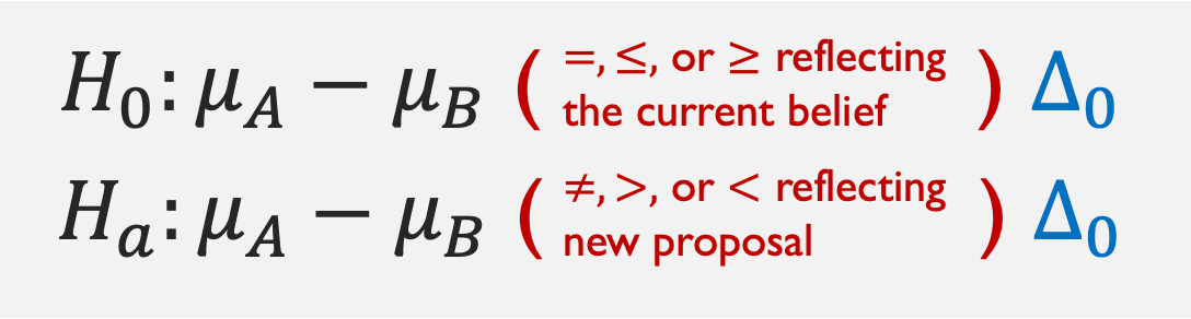
Fig. 11.1 Template for independent two-sample hypotheses
We denote the null value for a difference with \(\Delta_0\), using the Greek letter “Delta”.
Listing all possible combinations of null and alternative hypotheses from the template yields three distinct test types:
Upper-Tailed Hypothesis Test
Lower-Tailed Hypothesis Test
Two-Tailed Hypothesis Test
Special Case When the Null Value is Zero
In many cases, the test is on whether there is any difference between the two means, or whether one is larger or smaller than the other. These cases correspond to the special cases with \(\Delta_0 = 0\).
Upper-Tailed Test: “Is \(\mu_A\) greater than \(\mu_B\)?”
Lower-Tailed Test: “Is \(\mu_A\) less than \(\mu_B\)?”
Two-Tailed Test: “Is \(\mu_A\) different than \(\mu_B\)?”
Order Matters
The way we define the difference (\(\mu_A - \mu_B\) vs. \(\mu_B - \mu_A\)) determines the test type. To avoid confusion, clearly link the notation to the context and specify the order of subtraction.
11.1.4. Formulating Hypotheses for Paired Two-Sample Comparisons
Denote the samples from Populations A and B as:
respectively. Assume that each pair was assigned the same index. By taking the difference \(D_i = X_{A_i}-X_{Bi}\) for all \(i=1,2, \cdots, n,\) we obtain a single sample of \(n\) pair-wise differences. Hypothesis tests are then performed on the true mean of the differences, \(\mu_D,\) using one of the three possible formulations:
Upper-Tailed Hypothesis Test
Lower-Tailed Hypothesis Test
Two-Tailed Hypothesis Test
As in the independent analysis, the special cases with \(\Delta_0=0\) correspond to research questions about the direction of the difference (positive or negative) or about the existence of any difference at all.
Specifying the Order of Subtraction is Crucial for Paired Analysis ‼️
In paired two-sample analyses, clarifying the order of subtraction is especially important because the information is not apparent in the hypotheses. The related statement should be included in the first of the four steps of hypothesis testing, as part of parameter definition.
11.1.5. Bringing It All Together
Key Takeaways 📝
Two-sample procedures answer questions about differences between populations or treatments.
When the samples are independent, the two true means \(\mu_A\) and \(\mu_B\) are compared directly.
In paired samples, sampling on one side significantly influences sampling probabilities in the other. For their comparative analysis, the two-sample data is transformed to a single sample of differences \(D_i = X_{Ai} - X_{Bi}.\) The central parameter is the mean of the differences, \(\mu_D\).
11.1.6. Exercises
Exercise 1: Identifying Independent vs Paired Samples
For each research scenario, determine whether an independent or paired two-sample procedure is appropriate. Explain your reasoning.
Comparing fuel efficiency between two different car models by testing 30 vehicles of each model.
Measuring blood pressure before and after administering a new medication to the same 25 patients.
Comparing algorithm runtime by running Algorithm A on 15 datasets and Algorithm B on 15 different datasets.
Testing whether a tutoring program improves test scores by comparing pre-test and post-test results for 40 students.
Comparing tensile strength of steel produced by two different manufacturing processes, with 20 samples from each process.
Evaluating two different software optimization techniques by applying both to the same 12 programs and measuring execution time.
Solution
Part (a): Independent
The 30 vehicles of Model A and 30 vehicles of Model B are separate groups with no natural pairing. Each car in one group has no specific connection to any car in the other group.
Part (b): Paired
Each patient serves as their own control—the “before” measurement is naturally paired with the “after” measurement for the same individual. This controls for individual variation in baseline blood pressure.
Part (c): Independent
Although both algorithms are being tested, they’re run on different datasets. There’s no natural pairing between a dataset used for Algorithm A and one used for Algorithm B.
Note: If both algorithms were run on the same datasets, this would become a paired design—a valuable approach for comparing algorithms because it controls for dataset-specific variation. Pairing is often a design choice.
Part (d): Paired
Each student’s pre-test score is paired with their post-test score. The same individual generates both measurements, creating natural pairs.
Part (e): Independent
The steel samples from Process A and Process B come from different production runs with no natural pairing structure. Sample sizes need not be equal.
Part (f): Paired
Both optimization techniques are applied to the same programs. The execution time under Technique A for Program 1 should be compared directly to the time under Technique B for Program 1, controlling for program-specific complexity.
Exercise 2: Notation Practice
A quality engineer compares the precision of two measurement instruments. Instrument A was used for 18 measurements with mean 50.2 and standard deviation 2.1. Instrument B was used for 22 measurements with mean 49.8 and standard deviation 2.5.
Identify and write all the relevant notation: \(n_A, n_B, \bar{x}_A, \bar{x}_B, s_A, s_B\).
What is the parameter of interest if comparing independent populations?
Calculate the point estimate for the difference in population means.
If the true population standard deviations were known to be \(\sigma_A = 2.0\) and \(\sigma_B = 2.4\), write the formula for the standard error of \(\bar{X}_A - \bar{X}_B\).
Solution
Part (a): Notation
\(n_A = 18\) (sample size for Instrument A)
\(n_B = 22\) (sample size for Instrument B)
\(\bar{x}_A = 50.2\) (sample mean for Instrument A)
\(\bar{x}_B = 49.8\) (sample mean for Instrument B)
\(s_A = 2.1\) (sample standard deviation for Instrument A)
\(s_B = 2.5\) (sample standard deviation for Instrument B)
Part (b): Parameter of interest
\(\mu_A - \mu_B\), the difference between the true mean measurements from Instrument A and Instrument B.
Part (c): Point estimate
Part (d): Standard error formula
Exercise 3: Writing Hypotheses for Independent Samples
For each research question, write the appropriate null and alternative hypotheses. Define your parameters clearly.
A pharmaceutical company wants to test whether their new pain reliever provides faster relief than the current market leader.
An engineer wants to determine if two assembly lines produce components with different mean weights.
A researcher suspects that students using a new study app score at least 5 points higher on average than students using traditional methods.
A data scientist wants to test whether the mean response time of Server A is less than that of Server B.
Solution
Part (a): Pain reliever comparison
Let \(\mu_{new}\) = true mean time to pain relief (minutes) for the new drug. Let \(\mu_{current}\) = true mean time to pain relief (minutes) for the current market leader.
“Faster relief” means smaller time for the new drug:
Part (b): Assembly line weights
Let \(\mu_A\) = true mean weight of components from Line A. Let \(\mu_B\) = true mean weight of components from Line B.
Testing for any difference:
Part (c): Study app effectiveness
Let \(\mu_{app}\) = true mean exam score for students using the app. Let \(\mu_{trad}\) = true mean exam score for students using traditional methods.
Testing if the app improves scores by at least 5 points:
Note: Here \(\Delta_0 = 5\), not 0.
Part (d): Server response times
Let \(\mu_A\) = true mean response time for Server A. Let \(\mu_B\) = true mean response time for Server B.
Testing if Server A is faster (lower time):
Exercise 4: Writing Hypotheses for Paired Samples
For each paired scenario, define the difference appropriately and write the hypotheses.
A fitness trainer measures clients’ resting heart rate before and after a 12-week exercise program. The trainer expects the program to lower heart rate.
A software company tests response time of their application before and after a code optimization. They want to know if there’s any change.
An agricultural researcher applies two fertilizers to adjacent plots from the same field and measures crop yield. They want to test if Fertilizer A produces higher yields than Fertilizer B.
Solution
Part (a): Exercise program and heart rate
Define: \(D_i = \text{Heart Rate}_{\text{before}} - \text{Heart Rate}_{\text{after}}\) for each client.
Let \(\mu_D\) = true mean difference in heart rate (before - after).
If the program lowers heart rate, then “before” > “after”, so \(D > 0\):
Part (b): Code optimization
Define: \(D_i = \text{Response Time}_{\text{before}} - \text{Response Time}_{\text{after}}\).
Let \(\mu_D\) = true mean difference in response time.
Testing for any change (two-sided):
Part (c): Fertilizer comparison
Define: \(D_i = \text{Yield}_A - \text{Yield}_B\) for each paired plot.
Let \(\mu_D\) = true mean difference in yield (A - B).
If Fertilizer A produces higher yields, then \(D > 0\):
Exercise 5: Order of Subtraction Matters
A clinical trial compares a new treatment (N) versus a placebo (P) for reducing cholesterol levels.
If the difference is defined as \(D = X_N - X_P\) and researchers expect the new treatment to lower cholesterol more than the placebo, write the appropriate hypotheses.
If the difference is defined as \(D = X_P - X_N\) for the same research question, write the appropriate hypotheses.
Suppose \(\bar{d} = -15\) mg/dL when using definition (a). What would \(\bar{d}\) be using definition (b)?
Explain why it’s crucial to clearly specify the order of subtraction in Step 1 of hypothesis testing.
Solution
Part (a): D = Treatment - Placebo
If the treatment lowers cholesterol more than placebo, then patients on treatment have lower cholesterol levels, so \(X_N < X_P\), meaning \(D = X_N - X_P < 0\).
Part (b): D = Placebo - Treatment
With this definition, if treatment is more effective (lower cholesterol), then \(X_P > X_N\), so \(D = X_P - X_N > 0\).
Part (c): Relationship between definitions
If \(\bar{d} = -15\) using \(D = X_N - X_P\), then using \(D = X_P - X_N\):
The magnitude is the same; only the sign changes.
Part (d): Why specify the order
The order of subtraction determines:
The sign of the test statistic
Which tail of the distribution corresponds to the alternative hypothesis
How to interpret positive vs. negative differences
Without clear specification, results can be misinterpreted. A “positive difference” means opposite things depending on the definition.
Exercise 6: When is Δ₀ ≠ 0?
In most two-sample comparisons, we test whether there’s any difference (\(\Delta_0 = 0\)). However, sometimes we need a non-zero null value.
For each scenario, identify the appropriate \(\Delta_0\) and write the hypotheses.
A battery manufacturer claims their premium battery lasts at least 3 hours longer than their standard battery. A consumer group wants to test this claim.
A drug must reduce blood pressure by more than 10 mmHg compared to placebo to be considered clinically significant. Researchers want to test if the drug meets this threshold.
Two machines are supposed to produce parts with the same mean diameter. Quality control will intervene if the means differ by more than 0.5 mm.
Solution
Part (a): Battery life claim
Let \(\mu_P\) = true mean battery life for premium battery. Let \(\mu_S\) = true mean battery life for standard battery.
The manufacturer claims \(\mu_P - \mu_S \geq 3\). The consumer group wants to disprove this claim.
\(\Delta_0 = 3\) hours
Part (b): Clinical significance threshold
Define \(Y\) = blood pressure reduction (baseline minus follow-up), so larger \(Y\) means more reduction.
Let \(\mu_{drug}\) = true mean reduction for drug group. Let \(\mu_{plac}\) = true mean reduction for placebo group.
Testing if the drug exceeds the 10 mmHg clinical threshold compared to placebo:
\(\Delta_0 = 10\) mmHg
Part (c): Machine calibration (tolerance problem)
Let \(\mu_1\) = true mean diameter from Machine 1. Let \(\mu_2\) = true mean diameter from Machine 2.
Quality control will intervene if \(|\mu_1 - \mu_2| > 0.5\) mm. This is a tolerance or equivalence-style problem.
Approach 1: Confidence Interval Method (Recommended for this course)
Construct a two-sided confidence interval for \(\mu_1 - \mu_2\) and check whether the entire interval falls within (−0.5, 0.5):
If the CI lies entirely within (−0.5, 0.5), the machines are acceptably similar.
If the CI extends beyond ±0.5 in either direction, intervention may be needed.
Note: This is not a standard “test at Δ₀ = 0” problem. Using Δ₀ = 0 tests whether the means are exactly equal, not whether they are “close enough.”
Approach 2: Two One-Sided Tests (TOST) - Beyond STAT 350
For formal equivalence testing, one would test:
H₀: \(\mu_1 - \mu_2 \leq -0.5\) vs. Hₐ: \(\mu_1 - \mu_2 > -0.5\), AND
H₀: \(\mu_1 - \mu_2 \geq 0.5\) vs. Hₐ: \(\mu_1 - \mu_2 < 0.5\)
If both are rejected, conclude equivalence within ±0.5 mm. This advanced method is not covered in STAT 350.
Exercise 7: Identifying the Correct Procedure
For each scenario, identify:
Whether to use independent or paired samples
The appropriate parameter (\(\mu_A - \mu_B\) or \(\mu_D\))
What additional assumptions might be needed
Comparing crash test ratings between SUVs and sedans (15 of each type tested).
Testing whether students perform differently on paper vs. computer-based exams by having 30 students take both versions.
Comparing customer satisfaction between two restaurant locations by surveying 50 customers at each location.
Evaluating a new keyboard design by measuring typing speed before and after users switch to the new keyboard.
Comparing the accuracy of two different machine learning models by testing both on the same 100 datasets.
Solution
Part (a): Crash test ratings
Procedure: Independent samples
Parameter: \(\mu_{SUV} - \mu_{sedan}\)
Assumptions: Independence between groups, approximate normality in each group (or large enough samples for CLT)
Part (b): Paper vs. computer exams
Procedure: Paired samples
Parameter: \(\mu_D\) where \(D_i = \text{Paper}_i - \text{Computer}_i\)
Assumptions: Independence between student pairs, normality of differences
Note: Order effects (which test taken first) should be balanced in the design.
Part (c): Restaurant satisfaction
Procedure: Independent samples
Parameter: \(\mu_A - \mu_B\) (satisfaction scores at Location A vs. B)
Assumptions: Independence within and between groups, approximate normality or large samples
Part (d): Keyboard typing speed
Procedure: Paired samples
Parameter: \(\mu_D\) where \(D_i = \text{New}_i - \text{Old}_i\)
Assumptions: Independence between users, normality of differences
Part (e): ML model accuracy
Procedure: Paired samples
Parameter: \(\mu_D\) where \(D_i = \text{Accuracy}_{Model1,i} - \text{Accuracy}_{Model2,i}\)
Assumptions: Independence between datasets, normality of differences
Pairing by dataset controls for variation in dataset difficulty.
Exercise 8: True/False Conceptual Questions
Determine whether each statement is True or False. Provide a brief justification.
In a paired two-sample design, the sample sizes must be equal.
For independent samples, \(\mu_A - \mu_B\) and \(\mu_B - \mu_A\) lead to the same hypothesis test conclusions.
Paired designs always have higher power than independent designs.
The order of subtraction in paired analysis affects the sign of the test statistic but not the p-value for a two-sided test.
If two populations are independent, we can still use a paired analysis if we arbitrarily pair observations.
The parameter \(\mu_D\) in paired analysis equals \(\mu_A - \mu_B\) in value.
Solution
True — In paired samples, each observation in Sample A is matched with exactly one observation in Sample B, so \(n_A = n_B = n\) necessarily.
True for two-sided tests; False for one-sided tests — For two-sided tests (Hₐ: μ_A ≠ μ_B), switching the order changes the sign of the test statistic but the p-value remains the same since we consider both tails. For one-sided tests, reversing the subtraction reverses the direction of the alternative hypothesis, which can lead to opposite conclusions if not carefully adjusted.
False — Paired designs have higher power when there is substantial within-pair correlation. If pairs are essentially independent (low correlation), independent designs may have comparable or better power due to more degrees of freedom.
True — For two-sided tests, we use \(2P(|T| > |t_{TS}|)\). The absolute value makes the p-value the same regardless of sign.
False — Arbitrary pairing of independent observations does not create meaningful structure. It would reduce degrees of freedom (\(n-1\) instead of \(n_A + n_B - 2\)) without the benefit of controlling for variability, resulting in power loss.
True — \(\mu_D = E[D_i] = E[X_{Ai} - X_{Bi}] = \mu_A - \mu_B\). The expected value of the differences equals the difference of expected values.
Exercise 9: Practical Design Considerations
A biomedical engineer wants to compare the accuracy of two glucose monitoring devices. They have access to 40 patients.
Describe how to implement an independent samples design.
Describe how to implement a paired samples design.
What are the advantages of the paired design in this context?
What are potential drawbacks of the paired design?
Which design would you recommend and why?
Solution
Part (a): Independent samples design
Randomly assign 20 patients to use Device A
Randomly assign 20 patients to use Device B
Compare mean accuracy between the two independent groups
Part (b): Paired samples design
Have all 40 patients use both Device A and Device B
For each patient, calculate \(D_i = \text{Accuracy}_A - \text{Accuracy}_B\)
Analyze the differences using one-sample t-procedures
Part (c): Advantages of paired design
Controls for patient variability: Factors like blood glucose variability, skin type, and activity level affect both measurements equally and cancel out when differencing.
More powerful: By eliminating between-patient variation, the paired design can detect smaller differences.
Requires fewer patients: With proper pairing, 40 patients in a paired design may have more power than 40 patients split into two independent groups.
Part (d): Potential drawbacks
Carryover effects: If using one device affects the reading of the other (e.g., skin irritation), results may be biased.
Order effects: The order of device use should be randomized and balanced.
Time/cost: Each patient must be tested with both devices, potentially doubling measurement time.
Dropouts: If a patient drops out after using only one device, that data point is lost entirely.
Part (e): Recommendation
The paired design is recommended because:
Patient-to-patient variability in glucose levels is likely substantial
Both devices can be tested on the same blood sample or close in time
This controls for a major source of variability
To address drawbacks, randomize the order of device use and balance it across patients.
11.1.7. Additional Practice Problems
True/False Questions (1 point each)
Independent two-sample procedures require equal sample sizes.
Ⓣ or Ⓕ
In a paired design, observations within each pair are typically correlated.
Ⓣ or Ⓕ
The null value \(\Delta_0\) must always equal zero.
Ⓣ or Ⓕ
Before-and-after studies always require paired analysis.
Ⓣ or Ⓕ
In paired designs, \(\bar{d}\) always equals \(\bar{x}_A - \bar{x}_B\) when all pairs are complete.
Ⓣ or Ⓕ
Paired procedures have degrees of freedom \(n_A + n_B - 2\).
Ⓣ or Ⓕ
Multiple Choice Questions (2 points each)
Which scenario is best suited for a paired two-sample analysis?
Ⓐ Comparing average height between male and female students
Ⓑ Comparing test scores before and after a training program for the same employees
Ⓒ Comparing customer satisfaction at two different stores
Ⓓ Comparing defect rates between two manufacturing plants
For independent samples, the parameter of interest is:
Ⓐ \(\mu_D\)
Ⓑ \(\mu_A - \mu_B\)
Ⓒ \(\sigma_A - \sigma_B\)
Ⓓ \(\bar{X}_A - \bar{X}_B\)
When should \(\Delta_0 \neq 0\) be used in the hypotheses?
Ⓐ When sample sizes are unequal
Ⓑ When testing for a specific minimum difference
Ⓒ When using paired samples
Ⓓ When population variances are unknown
A key advantage of paired designs over independent designs is:
Ⓐ Larger degrees of freedom
Ⓑ Control of extraneous variability
Ⓒ Unequal sample sizes are allowed
Ⓓ No assumptions are required
In a paired analysis where \(D_i = X_{Ai} - X_{Bi}\), if \(\mu_D > 0\), then:
Ⓐ Population A has a smaller mean than Population B
Ⓑ Population A has a larger mean than Population B
Ⓒ The populations have equal means
Ⓓ Cannot be determined without more information
Which assumption is required for independent two-sample procedures but NOT for paired procedures?
Ⓐ Normality of the sampling distribution
Ⓑ Independence between the two samples
Ⓒ Random sampling
Ⓓ Known population means
Answers to Practice Problems
True/False Answers:
False — Independent samples can have different sizes (\(n_A \neq n_B\)).
True — The whole point of pairing is that observations are linked, typically creating positive correlation.
False — \(\Delta_0\) can be any value based on the research question (e.g., testing if difference exceeds 5 points).
False — “Before and after” studies only require paired analysis when the same individuals are measured at both times. If different individuals are measured before and after an intervention period (e.g., repeated cross-sections), independent samples methods apply.
True — When all pairs are complete, \(\bar{d} = \bar{x}_A - \bar{x}_B\) algebraically. However, in paired designs the primary parameter is \(\mu_D\), and the standard error is computed from the differences, not from the two samples separately.
False — Paired procedures have \(df = n - 1\) where n is the number of pairs.
Multiple Choice Answers:
Ⓑ — Same employees measured twice creates natural pairing.
Ⓑ — The difference in population means is the parameter; \(\bar{X}_A - \bar{X}_B\) is the estimator.
Ⓑ — Non-zero null values test for specific minimum or maximum differences.
Ⓑ — Pairing controls for individual/subject variability.
Ⓑ — If \(\mu_D = \mu_A - \mu_B > 0\), then \(\mu_A > \mu_B\).
Ⓑ — Independent procedures require the two samples to be independent; paired procedures require independence between pairs, not between the two measurements within a pair.