5.6. The Binomial Distribution

Certain patterns in probability occur so frequently that they deserve special attention. When we flip coins repeatedly, test multiple products for defects, or survey people about their preferences, we encounter the same underlying structure: a fixed number of independent trials, each with two possible outcomes. The binomial distribution captures this common scenario, providing us with ready-made formulas that eliminate the need to build probability models from scratch every time.

Road Map 🧭

• Identify when to use the binomial distribution through the BInS criteria.

• Master the binomial probability mass function and its parameters.

• Calculate expected value and variance using distribution properties.

• Apply binomial models to real-world counting problems.

• Connect binomial random variables to sums of independent Bernoulli trials.

5.6.1. Binomial Experiments

The binomial distribution emerges naturally when we perform the same basic experiment multiple times under controlled conditions. Think about flipping a coin ten times and counting heads, or testing twenty manufactured items for defects. These scenarios share a common structure that statisticians have studied extensively.

The BInS Criteria

A binomial experiment must satisfy four key properties, which we can remember using the acronym BInS:

The BInS checklist
Letter	Word	Meaning
B	Binary	Each trial has exactly two possible outcomes (success & failure).
I	Independent	Outcomes of different trials don’t influence one another.
n	Fixed (n) trials	The number of trials is set in advance.
S	Same (p)	The probability of success is identical for every trial.

Examples💡: Identifying a Binomial Experiment throuhg BInS

For each given scenario, determine whether the experiment fits the BInS criteria.

Example 1: Rolling a Die

Suppose we roll a fair four-sided die five times and observe whether each outcome is a 1 or not.

• Binary: Each roll either shows a 1 (success) or doesn’t (failure). ✓

• Independent: Each roll doesn’t affect subsequent rolls. ✓

• n-trials: We perform exactly 5 rolls. ✓

• Success: The probability of rolling a 1 remains 1/4 on every trial. ✓

This satisfies all BInS criteria, so it’s a binomial experiment.

Example 2: Drug Trial

Twenty patients with the same condition receive either a drug or placebo, and we measure whether the treatment is effective.

• Binary: This seems binary (effective/not effective), but there’s more complexity since patients are given different types of of treatment.

• Independent: Patient outcomes are independent. ✓

• n-trials: We have 20 patients ✓

• Success: The success probabilities may ore may not be the same for different patients, depending on the effectiveness of the drug. ❌

The experiment is not a binomial experiment.

Example 3: Quality Control

We randomly sample 15 products from an assembly line using different machines and classify each as acceptable or not acceptable.

• Binary: Each product is either acceptable or not. ✓

• Independent: Random sampling makes outcomes independent. ✓

• n-trials: We test exactly 15 products. ✓

• Success: Different machines may have different success rates ❌

This is not a binomial experiment.

Example 4: A different drug trial

A pharmaceutical company has developed a new medication for a common illness. In a clinical trial, 10 randomly selected patients receive the new medication to see if they recover within a fixed amount of time.

• Binary: Each patient either recovers or doesn’t. ✓

• Independent: One patient’s recovery doesn’t affect another’s. ✓

• n-trials: We observe exactly 10 patients. ✓

• Success: Recovery probability remains 0.3 for each patient. ✓

This is a binomial experiment.

5.6.2. The Binomial Distribution

When an experiment satisfies the BInS criteria, we can model the number of successes using a binomial distribution.

Definition

A binomial random variable \(X\) maps each outcome in a binomial experiment to the number of successes in \(n\) trials. We write this as:

\[X \sim \text{Bin}(n, p)\]

where

• \(n\) a positive integer representing the number of trials and

• \(p \in [0,1]\) is the probability of success on each trial.

Parameters

The set of quantities that specify a complete PMF in a known family of distributions are called parameters. \(n\) and \(p\) are the parameters of binomial distribution.

Probability Mass Function

The binomial PMF gives us the probability of exactly \(x\) successes in \(n\) trials:

\[p_X(x) = \binom{n}{x} p^x (1-p)^{n-x}\]

for \(x \in \text{supp}(X) = \{0, 1, 2, ..., n\}\).

This formula has three components:

1. Combinations:

   \(\binom{n}{x} = \frac{n!}{x!(n-x)!}\) counts the number of ways to arrange \(x\) successes among \(n\) trials.

2. Success probability:

   \(p^x\) accounts for the probability of getting exactly \(x\) successes.

3. Failure probability:

   \((1-p)^{n-x}\) accounts for the probability of getting \((n-x)\) failures.

The beauty of this formula lies in its generality. Once we know \(n\) and \(p\), we can calculate the probability for any number of successes without listing all possible outcomes.

Validating the binomial PMF

It is clear that for each \(x \in \text{supp}(X)\), \(p_X(x)\) gives a non-negative value, since the three components which make up its formula are non-negative. By verifying these terms sum to 1, we will also be able to argue that each \(p_X(x)\) is at most 1.

We compute the sum of all \(p_X(x)\) terms using the binomial theorem:

\[\sum_{x=0}^{n} \binom{n}{x} p^x (1-p)^{n-x} = (p + (1-p))^n = 1^n = 1.\]

So, the binomial PMF satsifies both conditions for validity.

5.6.3. Expected Value and Variance: Building from Bernoulli Trials

Rather than deriving the expected value and variance from the PMF directly, we can use a clever approach that connects the binomial distribution to simpler building blocks.

Bernoulli Random Variables

A Bernoulli random variable \(B\) represents the outcome of a single trial in a binomial experiment:

\[\begin{split}B = \begin{cases} 1 & \text{with probability } p \\ 0 & \text{with probability } 1-p \end{cases}\end{split}\]

For this simple random variable:

\[\begin{split}E[B] &= 1 \cdot p + 0 \cdot (1-p) = p, \\ E[B^2] &= 1^2 \cdot p + 0^2 \cdot (1-p) = p, \\ \text{Var}(B) &= E[B^2] - (E[B])^2 = p - p^2 = p(1-p).\end{split}\]

Connecting Bernoulli to Binomial

A binomial random variable is simply the sum of \(n\) independent Bernoulli trials:

\[X = B_1 + B_2 + \cdots + B_n\]

where each \(B_i\) represents the \(i\)-th trial.

Using the linearity of expectation:

\[E[X] = E[B_1 + B_2 + \cdots + B_n] = E[B_1] + E[B_2] + \cdots + E[B_n] = np\]

Since the trials are independent, we can add their variances:

\[\text{Var}(X) = \text{Var}(B_1) + \text{Var}(B_2) + \cdots + \text{Var}(B_n) = np(1-p)\]

Summary of Binomial Distribution Properties

For \(X \sim Bin(n, p)\):

\[\begin{split}&\mu_X = E[X] = np \\ &\sigma_X^2 = \text{Var}(X) = np(1-p) \\ &\sigma_X = \sqrt{np(1-p)}\end{split}\]

These formulas make intuitive sense.

• If we perform \(n\) trials with probability \(p\) of success each time, we expect about \(np\) successes on average.

• The variance reflects that we get maximum uncertainty when \(p = 0.5\) (each trial is equally likely to succeed or fail) and minimum uncertainty when \(p\) is close to 0 or 1.

5.6.4. Visualizing Binomial Distributions

The shape of a binomial distribution depends heavily on its parameters. Let’s examine how changing \(p\) affects the distribution when \(n = 10\):

Low Success Probability (\(p = 0.1\))

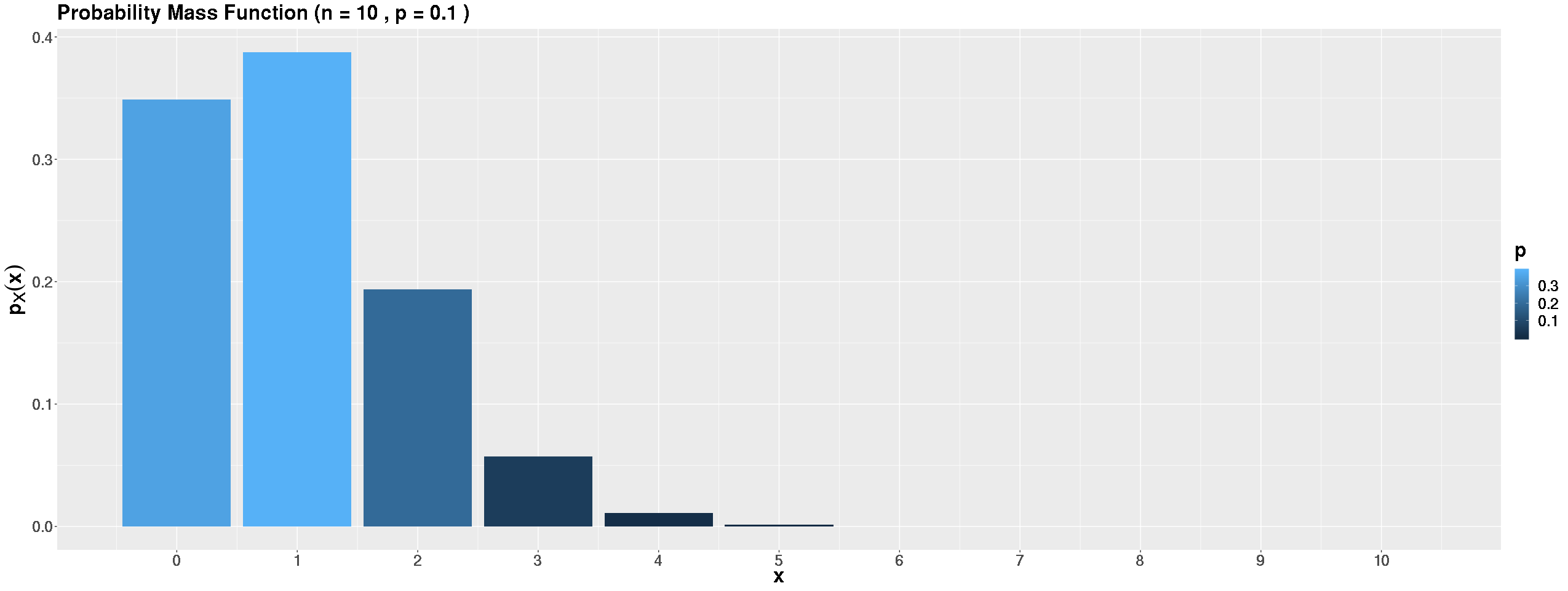
Fig. 5.6 p=0.1

When success is rare, most probability concentrates near zero. We expect 0.1 successes on average, so getting 0 or 1 success is most likely, with higher counts becoming increasingly rare.

Moderate Success Probability* (\(p = 0.25\))

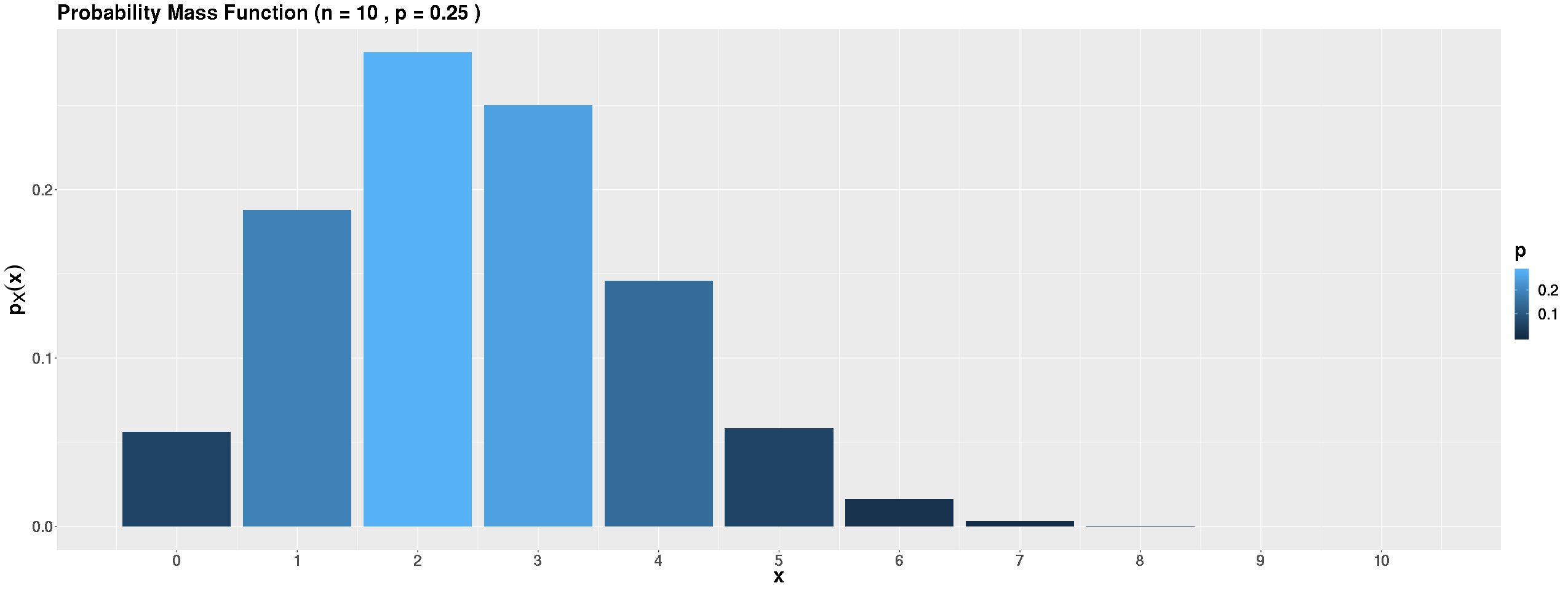
Fig. 5.7 p=0.25

As p increases, the distribution shifts right but remains skewed. We expect 2.5 successes on average, with reasonable probability spread across several values.

Equal Success and Failure (\(p = 0.5\))

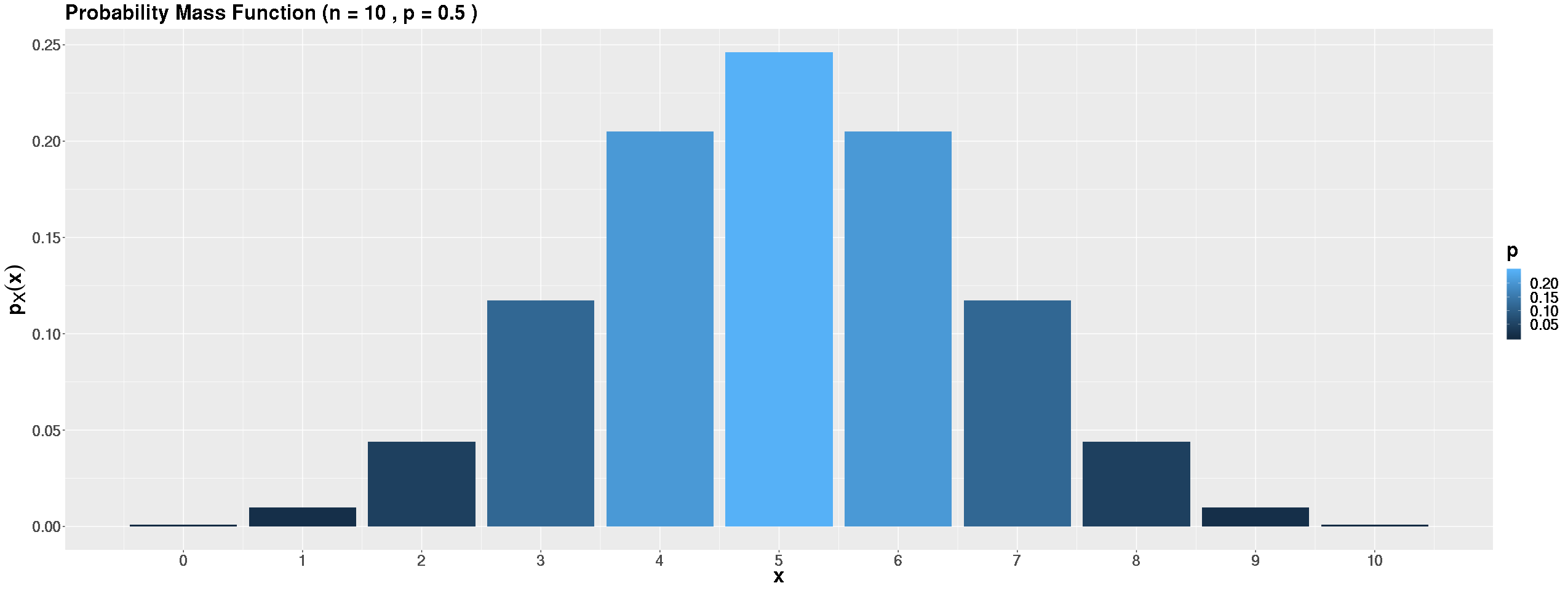
Fig. 5.8 p=0.5

When success and failure are equally likely, the distribution becomes symmetric around its mean of 5. This creates the classic bell-shaped pattern associated with binomial distributions.

High Success Probability (\(p = 0.9\))

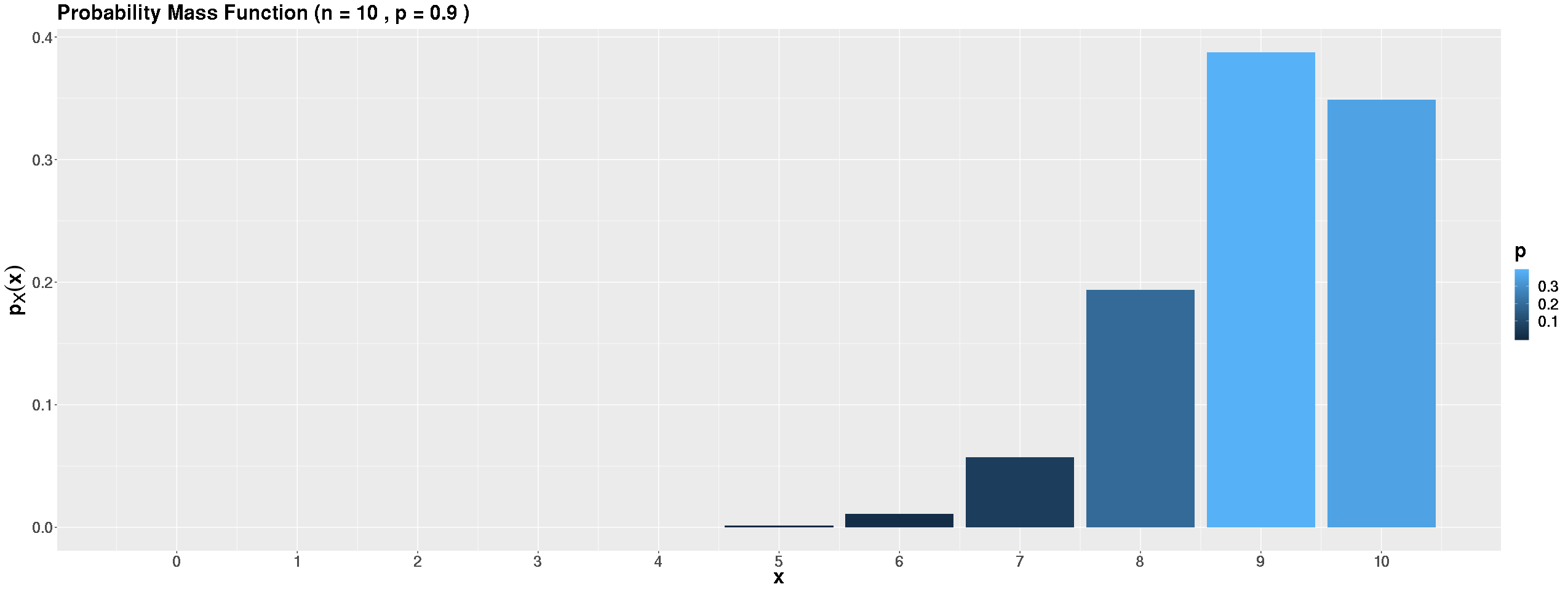
Fig. 5.9 p=0.9

When success is nearly certain, most probability concentrates near the maximum. We expect 9.9 successes, so getting 9 or 10 successes dominates the distribution.

Example💡: Evaluating a Medical Trial

A pharmaceutical company has developed a new medication for a common illness. Historical data shows that 30% of people with this illness recover naturally without treatment. In a clinical trial, 10 randomly selected patients received the new medication, 9 of which recovered. Is this strong evidence that the medication is effective, or could this result reasonably occur by chance alone?

Step 1: Confirm BInS Criteria

We confirmed that this is a binomial experiment through Case 4 of the first example in this section.

Step 2: Is the result realistic in nature?

If the number of recovered patients followed the natural recovery rate, we would have

\[X \sim Bin(10, 0.3).\]

What is the probability that we see a comparative or better recovery rate in nature than the current experiment? In other words, what is \(P(X\geq 9)\)?

\[\begin{split}P(X \geq 9) &= P(X=9) + P(X=10) \\ &= {10 \choose 9}(0.3)^9(0.7)^1 + {10 \choose 10}(0.3)^10(0.7)^0 \\ &\approx 0.000138 + 0.000006 = 0.000144\end{split}\]

Step 3: Interpreting the results

The probability of seeing 9 or more recoveries by chance alone is only about 0.000144, or roughly 1 in 7,000. This extremely small probability suggests that observing 9 recoveries is highly unlikely if the medication had no effect.

This analysis provides strong statistical evidence that the medication is effective, though we’d want to see results from larger, more carefully controlled studies before drawing definitive conclusions.

5.6.5. Bringin It All Together

Key Takeaways 📝

1. The binomial distribution models the number of successes in a set of independent and identical trials.

2. Use the BInS criteria to identify binomial situations: Binary outcomes, Independent trials, n:math:n fixed trials, and constant Success probability.

3. The binomial PMF \(p_X(x) = \binom{n}{x} p^x (1-p)^{n-x}\) combines combinatorics with basic probability principles.

4. Binomial random variables have simple rxpected value and variance formulas: \(E[X] = np\) and \(Var(X) = np(1-p)\), derived by viewing binomial variables as sums of Bernoulli trials.

5. Binomial distributions are symmetric when p = 0.5 and increasingly skewed as p approaches 0 or 1.

Exercises

1. Identifying Binomial Experiments: For each scenario, determine whether it represents a binomial experiment. If not, explain which criterion is violated.

   1. A basketball player shoots 20 free throws. Each shot is independent, and her historical free-throw percentage is 85%.

   2. Cards are drawn one by one from a standard deck without replacement until an ace is drawn.

   3. A survey asks 100 randomly selected voters whether they support a particular candidate.

   4. A quality inspector examines products coming off an assembly line until finding the first defective item.

2. Basic Probability Calculations: A fair coin is flipped 8 times. Let X be the number of heads.

   1. Identify the parameters n and p.

   2. Calculate P(X = 3).

   3. Find P(X ≤ 2).

   4. What are the mean and standard deviation of X?

3. Quality Control Application: A manufacturing process produces items that are 5% defective. If 25 items are randomly selected for inspection:

   1. What is the probability that exactly 2 items are defective?

   2. What is the probability that at most 1 item is defective?

   3. What is the expected number of defective items? What is the standard deviation?

   4. Would finding 5 defective items be considered unusual? Explain using probability.

4. Medical Testing: A diagnostic test correctly identifies a disease 90% of the time when the disease is present. If the test is performed on 12 patients who have the disease:

   1. What is the probability that all 12 tests are positive?

   2. What is the probability that at least 10 tests are positive?

   3. How many positive tests would you expect to see on average?

5. R Programming Practice: Use R to analyze the following scenarios:

   1. Simulate 1000 samples from Bin(15, 0.4) and create a histogram. How does the sample distribution compare to the theoretical distribution?

   2. For X ~ Bin(25, 0.2), find the value k such that P(X ≤ k) ≈ 0.95.

   3. Compare P(X = 10) for three binomial distributions: Bin(20, 0.5), Bin(30, 0.33), and Bin(40, 0.25). All have approximately the same mean—explain any differences in the probabilities.