Slides 📊

Download Chapter 6 slides (PPTX)

6.4. Normal Distribution

We now encounter the most important continuous distribution in all of statistics: the normal distribution.

Road Map 🧭

• Understand the historical development and significance of the normal distribution.

• Master the mathematical definition and properties of the normal PDF.

• Explore how the parameters \(\mu\) and \(\sigma\) control location and shape.

• Learn the famous empirical rule for quick probability estimates.

• Understand why standardization is essential for normal computations.

6.4.1. The Historical Legacy: From Gauss to Modern Statistics

The normal distribution carries a rich mathematical heritage spanning over two centuries. While often called the “Gaussian distribution” in honor of Carl Friedrich Gauss (1777-1855), the distribution’s development involved several brilliant mathematicians who recognized patterns in natural variation.

Gauss and the Method of Least Squares

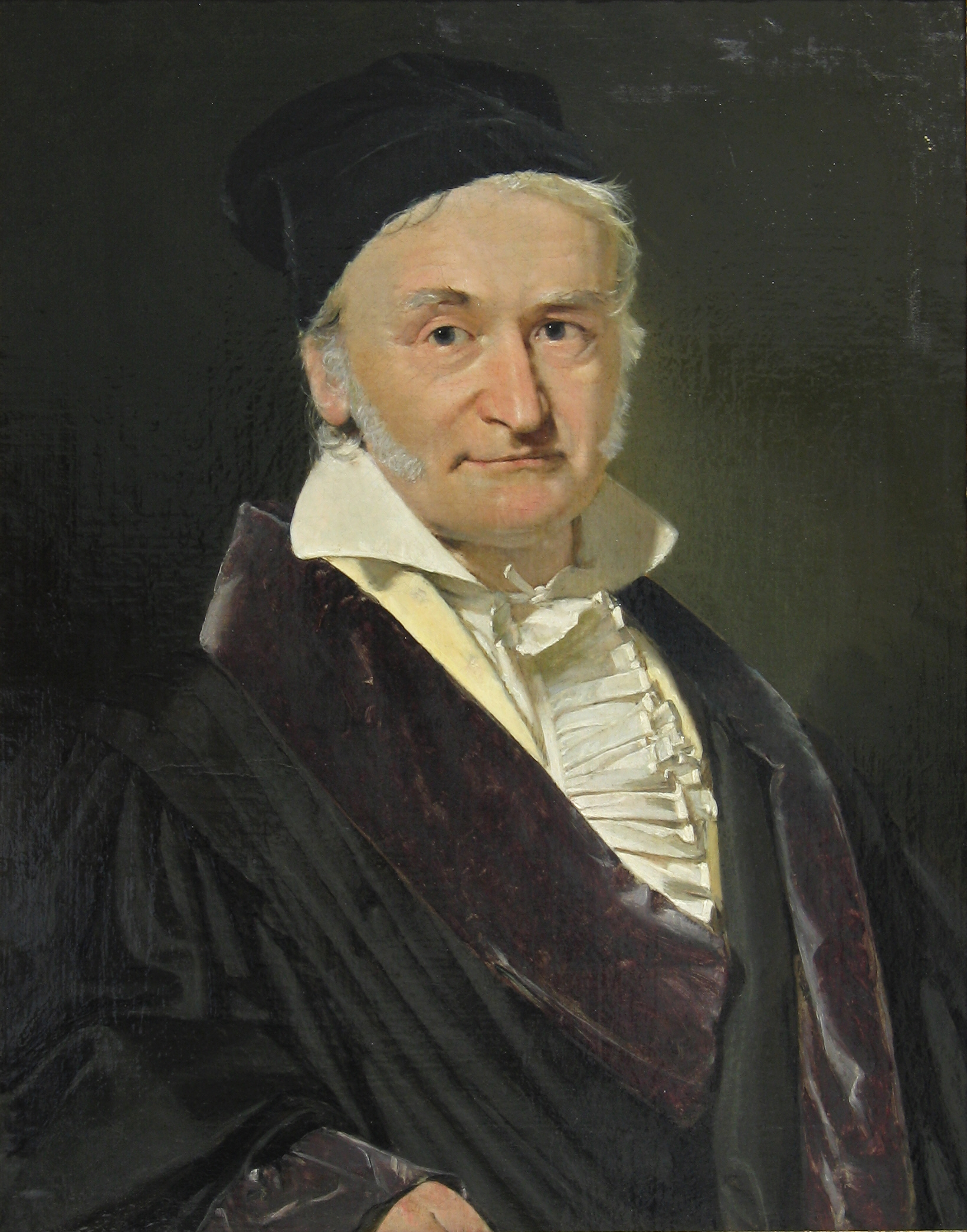
Fig. 6.25 Carl Friedrich Gauss (1777-1855)

In the late 1700s and early 1800s, Gauss was working on astronomical calculations and geodetic surveys—problems requiring precise measurements where small errors were inevitable. He sought to understand how these measurement errors behaved and how to optimally combine multiple measurements of the same quantity.

Gauss discovered that measurement errors followed a specific pattern: most errors were small and clustered around zero, with larger errors becoming increasingly rare. More importantly, he found that this error distribution had a particular exponential form with quadratic decay that optimized his least squares fitting procedure.

The Connection to Binomial Distributions

Gauss recognized that his continuous error distribution emerged as a limiting case of discrete binomial distributions. When the number of trials becomes very large while the probability of success becomes very small (in a specific balanced way), the jagged, discrete binomial distribution smooths into the graceful bell curve we now call the normal distribution.

This connection between discrete counting processes and continuous measurement errors revealed a profound unity in probability theory—the same mathematical structure appears whether we’re flipping coins or measuring stellar positions.

A Universal Pattern in Nature

What makes the normal distribution truly remarkable is its ubiquity. It describes not just measurement errors, but heights and weights of organisms, intelligence test scores, particle velocities in gases, and countless other natural phenomena. This universality isn’t coincidental—it emerges from a deep mathematical principle we’ll encounter later called the Central Limit Theorem.

6.4.2. The Mathematical Definition: Anatomy of the Bell Curve

Notation and Parameters

If a random variable \(X\) has a normal distribution, we write:

\[X \sim N(\mu, \sigma^2) \quad \text{or} \quad X \sim N(\mu, \sigma).\]

A normal random variable takes two parameters:

Parameter	Mean \(\mu\)	Standard Deviation \(\sigma\)
Possible values	\(\mu \in (-\infty, +\infty)\). It can be any real number.	\(\sigma >0\). It must be a postive value.
Interpretation	The location parameter. It represents the center of the distribution of \(X\).	The scale parameter. It represents how spread out the distribution of \(X\) is.
Effect on the appearance of the PDF	Slides the curve left or right, without changing the shape	Makes the graph tall and narrow (small \(\sigma\)) or wide and flat (large \(\sigma\)). It does not change the location of the center.

Variance or Standard Deviation?

It is standard to describe a normal distribution using either variance or standard deviation, but we must be explicit about which we’re using.

The constraints and interpretations of standard deviation transfer almost directly to variance. Variance must be a positive number, and it controls how wide the distribution is. The only difference is their scale—variance is in the squared scale, while standard deviation is on the same scale as \(X\).

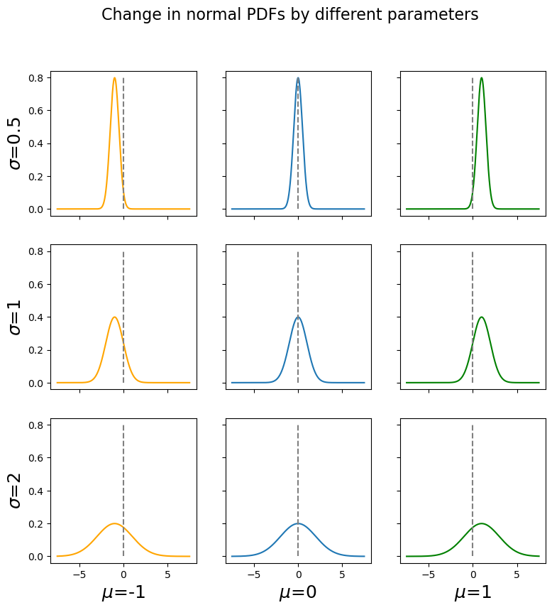
Fig. 6.26 How different values of μ and σ affect the normal distribution’s appearance

The Normal PDF

The PDF of a normal random variable \(X\) takes the form:

\[f_X(x) = \frac{1}{\sqrt{2\pi \sigma}} e^{-\frac{1}{2}\left(\frac{x-\mu}{\sigma}\right)^2} \quad \text{for all } x \in \mathbb{R}\]

This elegant formula contains several key components:

• The normalizing constant \(\frac{1}{\sqrt{2\pi \sigma}}\) ensures the total area under the curve equals 1.

• The exponential function \(e^{-(\cdot)}\) creates the smooth, continuous decay.

• The quadratic expression \(\left(\frac{x-\mu}{\sigma}\right)^2\) in the exponent produces the symmetric, bell-shaped curve.

• The parameters \(\mu\) and \(\sigma\) control the distribution’s location and spread.

Fundamental Properties

Regardless of its parameters, every normal distribution satisfies the following properties:

1. It is symmetrical about the mean \(\mu\).

2. It is unimodal with a single peak at \(x = \mu\).

3. Since the distribution is perfectly symmetric, the mean equals the median: \(\mu = \tilde{\mu}\).

4. It is bell-shaped with smooth, continuous curves.

5. The two tails approach but never reach zero as \(x \to \pm\infty\). This implies that \(\text{supp}(X) = (-\infty, +\infty)\).

6. The points where the normal curve changes from concave down to concave up (its inflection points) occur exactly at \(x = \mu - \sigma\) and \(x = \mu + \sigma\).

   

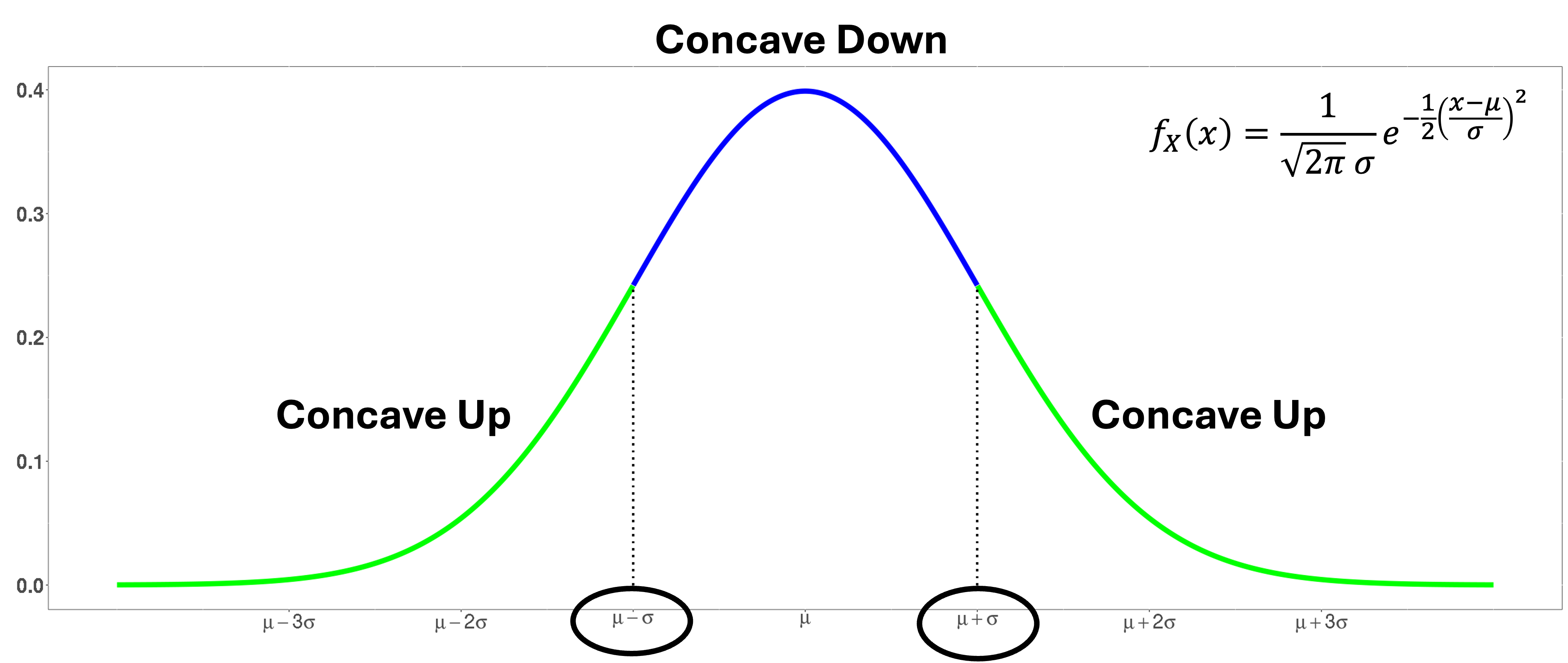
   Fig. 6.27 The normal curve changes concavity at exactly one standard deviation from the mean

6.4.3. The Empirical Rule: A Practical Tool

One of the most useful properties of normal distributions is that they all follow the same probability pattern, regardless of their specific parameter values. This universal pattern is called the empirical rule or 68-95-99.7 rule.

For any normal random variable \(X \sim N(\mu, \sigma)\),

1. 68% of the probability lies within one standard deviation from the mean: \(P(\mu - \sigma < X < \mu + \sigma) \approx 0.68\)

2. 95% of the probability lies within two standard deviations: \(P(\mu - 2\sigma < X < \mu + 2\sigma) \approx 0.95\)

3. 99.7% of the probability lies within three standard deviations: \(P(\mu - 3\sigma < X < \mu + 3\sigma) \approx 0.997\)

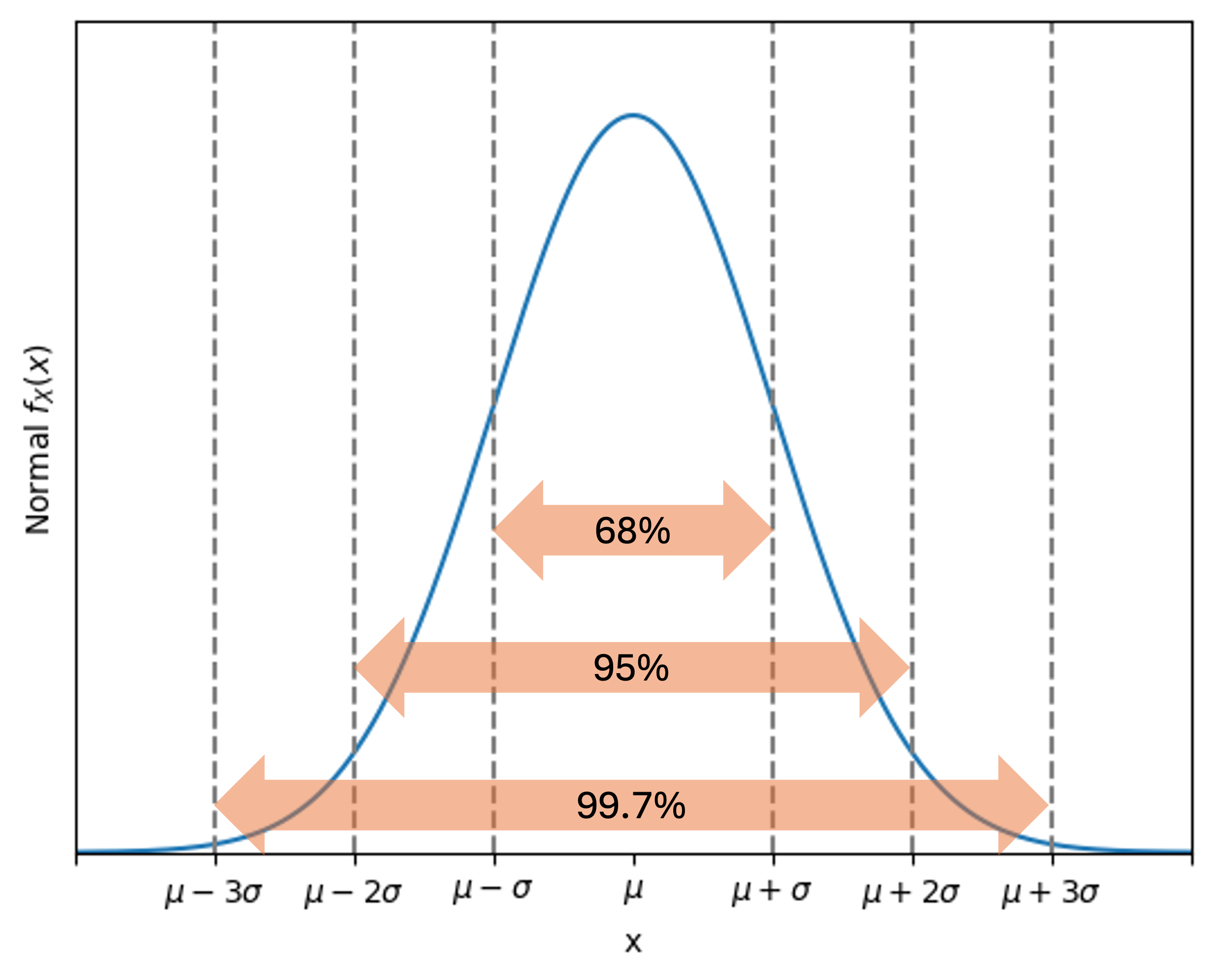
Fig. 6.28 The empirical rule provides quick probability estimates for any normal distribution

Extended Breakdown of the Empirical Rule

1. 34% of probability lies in each of \((\mu, \mu + \sigma)\) and \((\mu - \sigma, \mu)\)

   • Each interval is half of 68%.

2. 13.5% of probability lies in each of \((\mu + \sigma, \mu + 2\sigma)\) and \((\mu - 2\sigma, \mu - \sigma)\)

   • Each interval is half of 95%, minus an interval from #1.

3. 2.35% of probability lies in each of \((\mu + 2\sigma, \mu + 3\sigma)\) and \((\mu - 3\sigma, \mu - 2\sigma)\).

   • Each interval is half of 99.7%, minus an interval from #2 and an interval from #1.

4. 0.15% of probability lies beyond \(\mu + 3\sigma\) and another 0.15% beyond \(\mu - 3\sigma\).

   • Each region is half of 100% - 99.7%.

Insights from the Empirical Rule

• About 2/3 of values fall within one standard deviation of the mean.

• About 19 out of 20 values fall within two standard deviations.

• Nearly all values (99.7%) fall within three standard deviations.

Example💡: Computing Normal Probabilities Using Empirical Rules

A chemical lab reports that the amount of active ingredient in a single tablet of a medication is normally distributed with a mean of 500 mg and a standard deviation of 5 mg.

Q1. What is the probability that a tablet contains between 490 mg and 505 mg of active ingredient?

\(490 = \mu - 2\sigma \text{ and } 505 = \mu + \sigma\). Therefore, we are looking for

\[P(\mu -2\sigma \leq X \leq \mu + \sigma)\]

There are many different ways to solve this using the empirical rule. One way is to view the probability as

\[P(\mu -2\sigma \leq X \leq \mu + 2\sigma) - P(\mu+\sigma \leq X \leq \mu +2\sigma)\]

The first term is approximately 0.95 by the empirical rule, and the second term is approximately 0.135. Then finally,

\[P(\mu -2\sigma \leq X \leq \mu + \sigma) \approx 0.95 - 0.135 = 0.815\]

6.4.4. The Standard Normal Distribution: The Foundation of All Normal Computations

While normal distributions can have any mean and standard deviation, there’s one particular normal distribution that serves as the foundation for all normal probability calculations.

Definition of the Standard Normal Distribution

The standard normal distribution is the normal distribution with mean 0 and standard deviation 1. When a random variable follows the standard normal distribution, we denote it with \(Z\) and write:

\[Z \sim N(0, 1)\]

Its PDF is obtained by plugging in 0 and 1 for \(\mu\) and \(\sigma\), respectively, in the general form:

\[f_Z(z) = \frac{1}{\sqrt{2\pi}} e^{-\frac{z^2}{2}} \quad \text{for all } z \in \mathbb{R}\]

Because the standard normal is so important, it also gets special notations for its PDF and CDF:

• PDF: \(\phi(z) = f_Z(z)\) (lowercase Greek letter phi)

• CDF: \(\Phi(z) = P(Z \leq z)\) (uppercase Greek letter phi)

Standardization of Normal Random Variables

Any normal random variable can be converted to a standard normal random variable using the standardization formula:

\[Z = \frac{X - \mu}{\sigma}.\]

If \(X \sim N(\mu, \sigma)\), then \(Z \sim N(0, 1)\).

Why Standardization Works

1. Standardization re-centers the distribution at 0 by subtracting the mean from \(X\) .

2. It rescales the distribution to have unit variance by dividing \(X\) by its own standard deviation.

For a more concrete demonstration, we first need to know a special property of normal distribution:

• When a normal random variable is multiplied or added by a constant, the resulting random variable will still be normal, just with a new set of mean and variance parameters.

Since \(\mu\) and \(\sigma\) are constants, the operation on \(X\) to get to \(Z\) leaves us with another normal random variable. Also,

• \(E[Z] = E\left[\frac{X-\mu}{\sigma}\right]= \frac{E[X]-\mu}{\sigma} = \frac{\mu - \mu}{\sigma}=0\).

• \(\sigma^2[Z] = \text{Var}(Z) = \text{Var}\left(\frac{X-\mu}{\sigma}\right) = \frac{\text{Var}(X)}{\sigma^2}= \frac{\sigma^2}{\sigma^2} =1\).

Why Do We Standardize?

The fundamental problem with normal distributions is that their CDFs cannot be expressed in terms of elementary functions. There’s no simple formula for:

\[P(X\leq x) = \int_{-\infty}^{x} \frac{1}{\sqrt{2\pi \sigma}} e^{-\frac{1}{2}\left(\frac{t-\mu}{\sigma}\right)^2} dt\]

However, we can numerically approximate these integrals for the standard normal distribution and tabulate the results. Instead of creating tables of approximations for all possible pairs of parameters—which would be impossible—we standardize, so that we can refer to one table for any normal random variables.

6.4.5. Forward Problems: \(x\) to Probability

Now that we understand the theoretical foundation, let’s learn how to actually compute probabilities for normal distributions. Since we cannot integrate the normal PDF analytically, we rely on numerical approximations tabulated in standard normal tables.

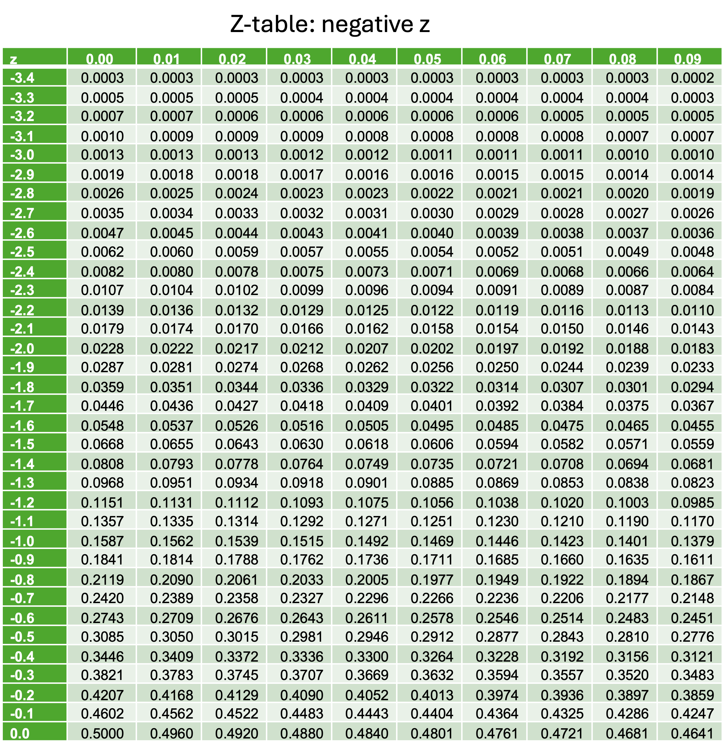
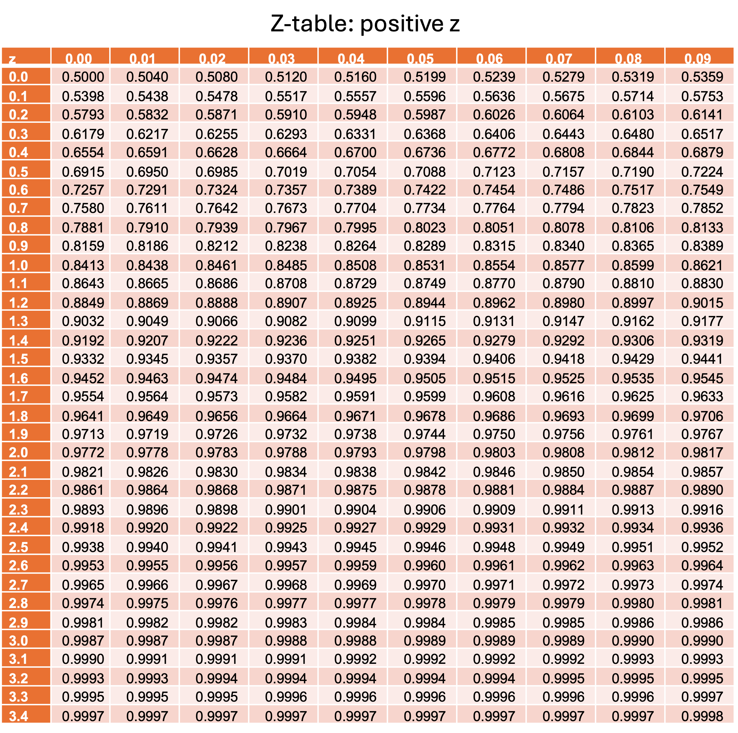
The Standard Normal Table (Z-Table)

Statisticians have computed high-precision numerical approximations for the standard normal CDF \(\Phi(z) = P(Z \leq z)\) and compiled them into tables. These tables typically provide probabilities accurate to four decimal places for z-values given to two decimal places.

For example, if we want to find \(P(Z \leq -1.38)\), first locate \(-1.3\) from the row labels. Then find the column with the label \(0.08\). The intersection of the row and the column gives the desired probability. \(P(Z \leq -1.38)=0.0838\).

The Strategy for Non-standard Normal RVs

We said we would apply the standardization technique to use the Z-table for any normal distributions. How will this work? The key steps are the following:

1. Recognize that subtracting the same value on both sides or multiplying by the same positive value on both sides does not change the truth of an (in)equality. It follows that the probability of the (in)equality also remains unchanged.

2. Using #1,

   \[P(X \leq a) = P\left(\frac{X-\mu}{\sigma} \leq \frac{a-\mu}{\sigma}\right) = P\left(Z \leq \frac{a-\mu}{\sigma}\right) = \Phi\left(\frac{a-\mu}{\sigma}\right).\]

   • \(\frac{a-\mu}{\sigma}\), the value obtained by standardizing \(a\), is called the z-score of \(a\).

The Strategy for Probabilities Which Do Not Match the CDF

We are often interested in probabilities which are not in the form \(\Phi(z) = P(Z \leq z)\).

• For “greater than” probabilities, use the complement rule: \(P(Z > z) = 1 - \Phi(z)\).

• For probabilities of intervals, use \(P(a < Z < b) = \Phi(b) - \Phi(a)\)

• Because the standard normal distribution is symmetric around zero, we have an additional tool: \(\Phi(-z) = 1 - \Phi(z)\) (Fig. 6.29).

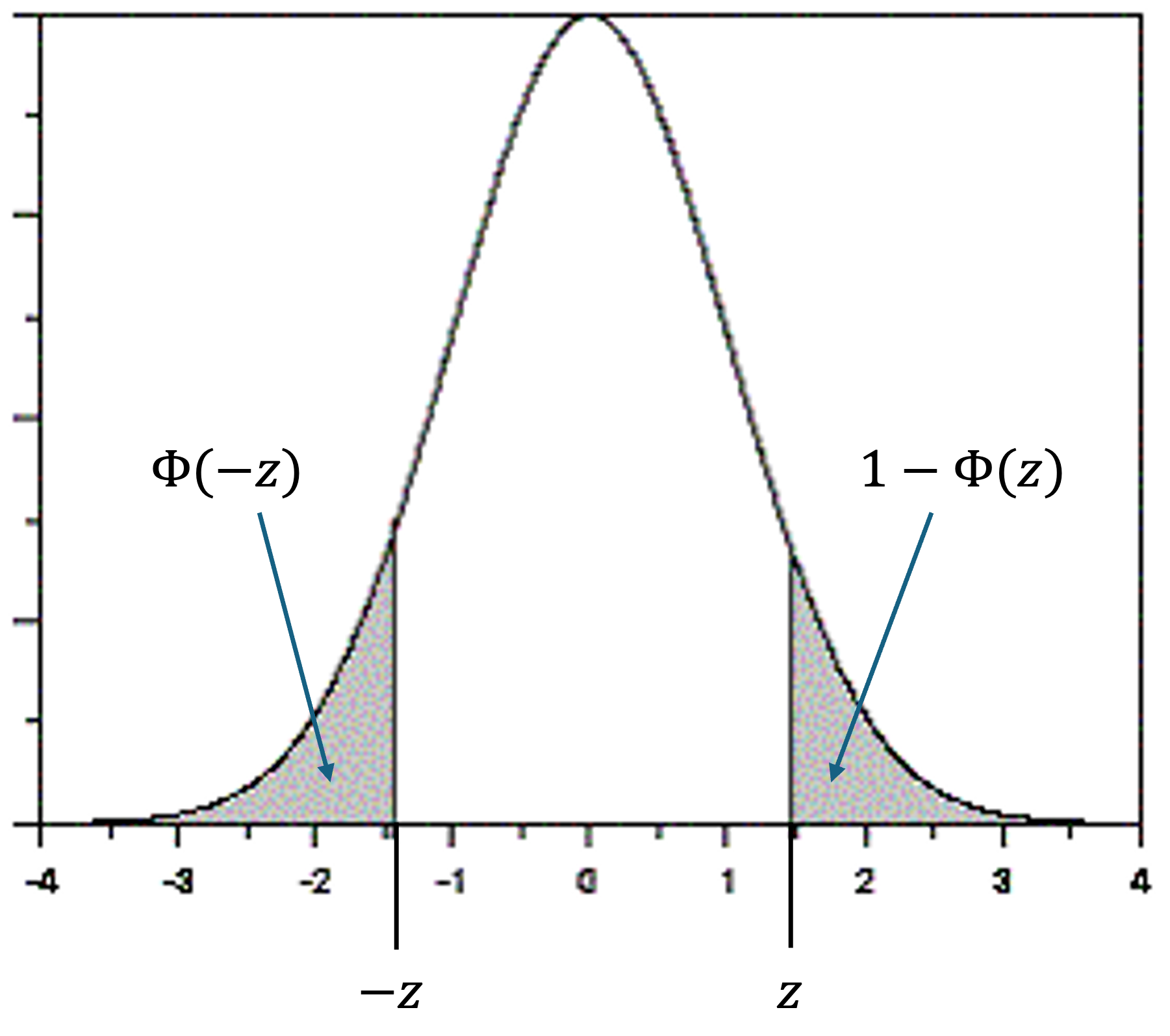
Fig. 6.29 Due to symmetry around zero, the two grey regions have equal probability.

Forward Problems

When a problem gives a value in the support and asks for a related probability, we call it a forward problem. The systematic approach is:

1. Identify the desired probability in correct probability notation. Sketch the region on a normal PDF plot if needed.

2. Standardize by converting \(x\) values to \(z\)-scores using \(z = \frac{x-\mu}{\sigma}\).

3. Modify the probability statement to an expression involving \(P(Z \leq z)\) so the Z-table can be used directly.

4. Round the z-score to two decimal places and look it up in the table.

5. Write your conclusion in the context of the problem.

Example💡: Systolic Blood Pressure

Systolic blood pressure readings for healthy adults, in mmHg, follow a normal distribution with \(\mu=112\) and \(\sigma^2= 100\). Find the probability that a randomly selected adult has blood pressure between 90 and 134 mmHg.

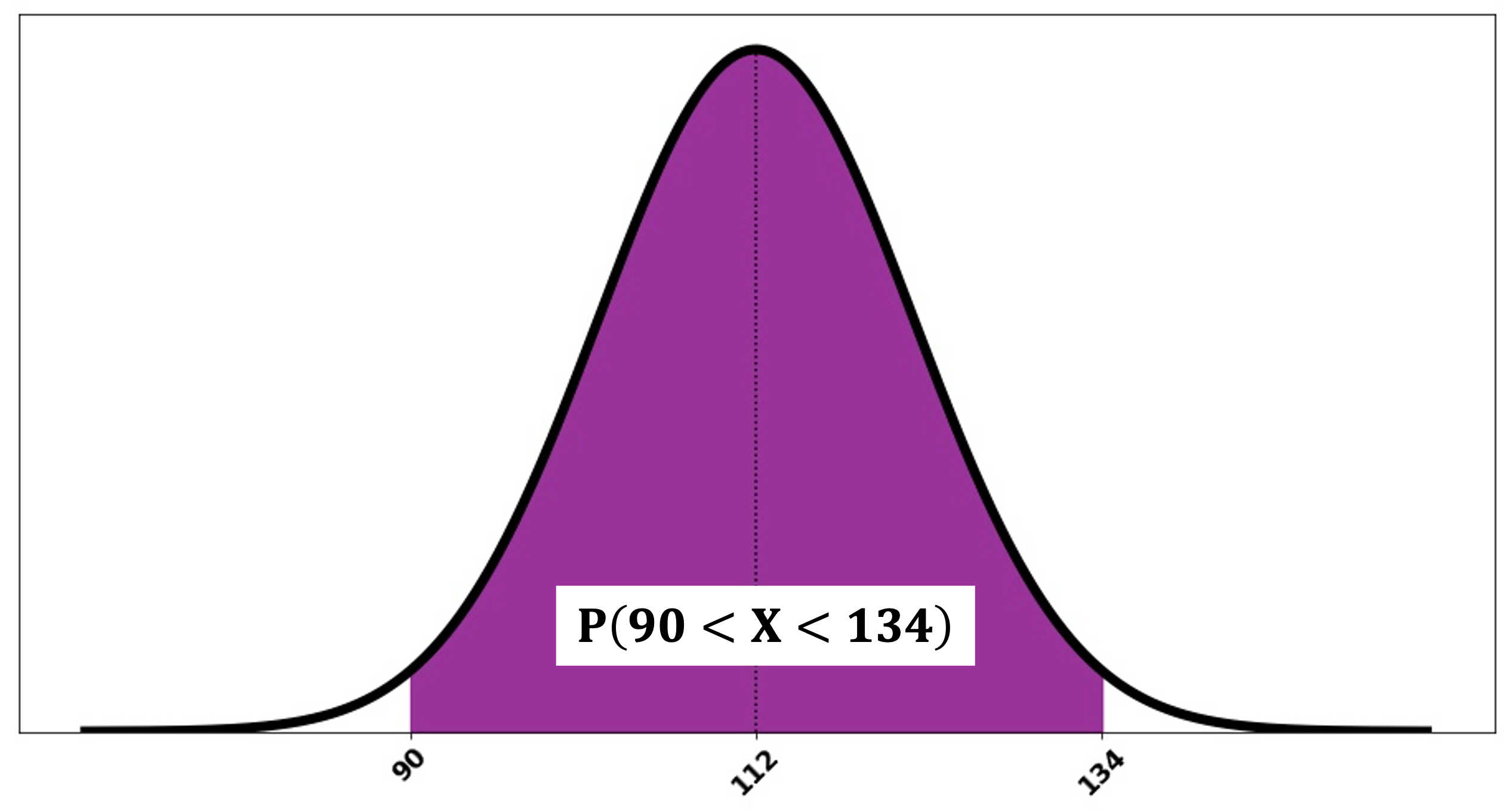
Fig. 6.30 A sketch of \(P(90 < X < 134)\)

• Step 1: Write the random variable and its distribution in correct notation

  Let \(X\) be the blood pressure readings for healthy adults. \(X \sim N(\mu=112, \sigma^2=100)\).

• Step 2: Find the correct probability statement

  We are looking for

  \[P(90 < X < 134) = P(X < 134) - P(X < 90).\]

  We need to find \(z_1\) and \(z_2\) such that \(P(X < 134) = P(Z< z_2)\) and \(P(X< 90)=P(Z< z_1)\).

• Step 3: Standardize to find \(z_1\) and \(z_2\)

  Note that the spread parameter is given as variance. We must use \(\sigma = \sqrt{100} = 10\) for standardization.

  \[z_1 = \frac{90 - 112}{10} = \frac{-22}{10} = -2.2 \text{ and } z_2 = \frac{134 - 112}{10} = \frac{22}{10} = 2.2\]

• Step 4: Convert to standard normal probability

  \[P(90 < X < 134) = P(Z< z_2) - P(Z< z_1) = \Phi(2.2) - \Phi(-2.2)\]

• Step 5: Use symmetry to simplify

  We can look up the CDF values for \(z_1=-2.2\) and \(z_2=2.2\) separately, but when the two \(z\)-scores are negatives of each other, we can also simplify the search step using \(\Phi(-2.2) = 1 - \Phi(2.2)\).

  \[P(-2.2 < Z < 2.2) = \Phi(2.2) - (1 - \Phi(2.2)) = 2\Phi(2.2) - 1\]

• Step 6: Look up in the Z-table and calculate the final answer

  From the Z-table: \(\Phi(2.2) = 0.9861\). Finally,

  \[P(90 < X < 134) = 2(0.9861) - 1 = 0.9722\]

  There is approximately 0.9722 probability that a randomly selected healthy adult will have systolic blood pressure between 90 and 134 mmHg.

6.4.6. Backward Problems: Probability to \(x\) (Percentile)

Backward problems reverse the process: given a probability, we must find the corresponding value (percentile) in the support.

Walkthrough of a Backward Problem

Consider a typical backward question:

• The gas price on a fixed date in State A follows normal distribution with mean $3.30 and standard deviation $0.12. If Gas Station B has a price higher than 63% of all gas stations in the state that day, what is the gas price in Gas Station B?

In this problem, a probability is given (63% or 0.63), and we are asked for the cutoff whose left region under the PDF has an area of 0.63. This cutoff is the 63th percentile of the gas price distribution.

To solve for this type of problems, we begin by setting up the correct probability statement.

\[P(X \leq x_{0.63}) = 0.63.\]

Standardize to get a probability statement in terms of \(Z\):

\[P(Z \leq \frac{x_{0.63}-\mu}{\sigma})=0.63.\]

The right-hand side of the inequality above now fits the definition of the 63th percentile of a standard normal random variable. That is,

\[z_{0.63} = \frac{x_{0.63}-\mu}{\sigma}.\]

We will look for \(z_{0.63}\) and convert back to \(x_{0.63}\) using this relationship.

To find \(z_{0.63}\), we locate 0.63 (or the value closest to it) in the main body of the table, then obtain the \(z\)- score from its margins. 0.6293 is the value closest to 0.63 in the main body, and its margins give us \(z_{0.63}=0.33\).

Converting back, \(x_{0.63} = \sigma z_{0.63} +\mu = (0.12)(0.33) + 3.3 = 3.3396\).

Finally, the price at Gas Station B is around $3.34.

Summary of the Key Steps

1. Identify the value you need to find using correct probability notation. Sketch the region if needed.

2. Find the z-score by first locating the probability in the body of the Z-table then going to its margins.

3. Convert the z-score to the original scale using \(x = \sigma z + \mu\).

4. Write your conclusion in the correct context.

Points That Require Special Attention

• Depending on the problem, the probability given may correspond to a right (upper) region rather than a left (lower) one under the PDF. Since percentiles are always defined in terms of the lower region, you need to make adjustments accordingly. For example, if Gas Station C has a price lower than 23 % of all other gas stations in the state, its price corresponds to the (100 – 23)th percentile.

• If the given probability does not have an exact match in the table, take the z-value for the closest entry. If it is exactly in the middle of two values on the table, take the average between the z-scores of the two entries.

Example💡: Systolic Blood Pressure, Continued

Continue with the RV of blood pressure measurements: \(X \sim N(\mu = 112, \sigma^2 = 100)\).

1. find the 95th percentile.

   We want to find \(x_{0.95}\) such that \(P(X \leq x_{0.95}) = 0.95\) First, find \(z_{0.95}\) such that \(\Phi(z_{0.95}) = 0.95\)

   In the body of the Z-table, we find that 0.9495 and 0.9505 are the closest to 0.95. Since 0.95 is exactly halfway between these values, we average the corresponding z-scores:

   \[z_{0.95} = \frac{1.64 + 1.65}{2} = 1.645.\]

   Converting to the original scale,

   \(x_{0.95} = \mu + \sigma z_{0.95} = 112 + 10(1.645) = 128.45\).

   Conclusion: The 95th percentile of systolic blood pressure is 128.45 mmHg. This means that 95% of healthy adults have blood pressure at or below this value.

2. Find the cutoffs for the middle 50% of blood pressure measurements. Using the cutoffs, also compute the interquartile range.

   

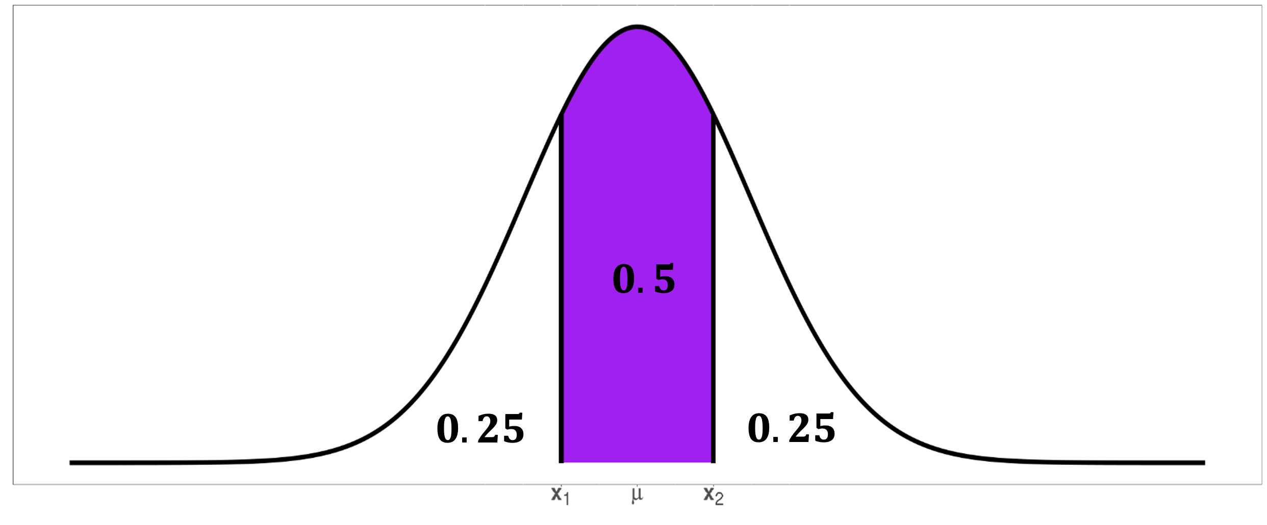
   Fig. 6.31 A sketch of problem 2

   We need to find two cutoffs: the 25th percentile and the 75th percentile.

   For the 25th percentile:

   • \(\Phi(z_{0.25}) = 0.25\)

   • From the table: \(z_{0.25} = -0.67\)

   • \(x_{0.25} = 112 + 10(-0.67) = 105.3\) mmHg

   For the 75th percentile:

   • \(\Phi(z_{0.75}) = 0.75\)

   • From the table (or using symmetry): \(z_{0.75} = 0.67\)

   • \(x_{0.75} = 112 + 10(0.67) = 118.7\) mmHg

   Conclusion: The middle 50% of systolic blood pressure readings fall between 105.3 and 118.7 mmHg. The interquartile range is \(118.7 - 105.3 = 13.4\) mmHg.

6.4.7. Proving the Theoretical Properties of Normal Distribution

Validity of the PDF

To establish that a normal PDF is legitimate, we must verify that it satisfies the two fundamental requirements for any probability density function.

Property 1: Non-Negativity

We need to show that \(f_X(x) \geq 0\) for all \(x\).

Since \(\sigma > 0\), we have \(\frac{1}{\sqrt{2\pi \sigma}} > 0\). The exponential function \(e^{-\frac{1}{2}\left(\frac{x-\mu}{\sigma}\right)^2}\) is always positive because:

• The exponent \(-\frac{1}{2}\left(\frac{x-\mu}{\sigma}\right)^2\) is always negative (or zero).

• \(e^{\text{negative number}}\) is always positive.

• \(e^0 = 1 > 0\).

Therefore, \(f_X(x) > 0\) for all \(x \in \mathbb{R}\). ✓

Property 2: Integration to Unity

We must prove that \(\int_{-\infty}^{\infty} f_X(x) \, dx = 1\).

Step 1: Change of Variables

Let \(z = \frac{x - \mu}{\sigma}\), so \(x = \sigma z + \mu\) and \(dx = \sigma \, dz\).

\(z = -\infty\) when \(x = -\infty\), and \(z = +\infty\) when \(x = +\infty\). The integral becomes:

\[I = \int_{-\infty}^{\infty} \frac{1}{\sqrt{2\pi \sigma}} e^{-\frac{1}{2}\left(\frac{x-\mu}{\sigma}\right)^2} dx = \int_{-\infty}^{\infty} \frac{1}{\sqrt{2\pi}} e^{-\frac{z^2}{2}} dz\]

Step 2: The Squaring Trick

This integral has no elementary antiderivative, so we use a clever approach. Let’s compute \(I^2\):

\[I^2 = \left(\int_{-\infty}^{\infty} \frac{1}{\sqrt{2\pi}} e^{-\frac{z^2}{2}} dz\right)\left(\int_{-\infty}^{\infty} \frac{1}{\sqrt{2\pi}} e^{-\frac{v^2}{2}} dv\right)\]

Since the integrals converge absolutely, we can rewrite this as a double integral:

\[I^2 = \int_{-\infty}^{\infty} \int_{-\infty}^{\infty} \frac{1}{2\pi} e^{-\frac{1}{2}(z^2 + v^2)} \, dz \, dv\]

Step 3: Polar Coordinate Transformation

Let:

• \(z = r\cos\theta\)

• \(v = r\sin\theta\)

• \(z^2 + v^2 = r^2\)

• \(dz \, dv = r \, dr \, d\theta\)

The integration limits become:

• \(r\): from 0 to \(\infty\)

• \(\theta\): from 0 to \(2\pi\)

Therefore:

\[I^2 = \int_0^{2\pi} \int_0^{\infty} \frac{1}{2\pi} e^{-\frac{r^2}{2}} \cdot r \, dr \, d\theta\]

Step 4: Separating the Integrals

\[I^2 = \frac{1}{2\pi} \int_0^{2\pi} d\theta \int_0^{\infty} r e^{-\frac{r^2}{2}} dr\]

The first integral gives us \(2\pi\). For the second integral, use substitution \(u = \frac{r^2}{2}\), so \(du = r \, dr\):

\[\int_0^{\infty} r e^{-\frac{r^2}{2}} dr = \int_0^{\infty} e^{-u} du = \left[-e^{-u}\right]_0^{\infty} = 0 - (-1) = 1\]

Step 5: Final Result

\[I^2 = \frac{1}{2\pi} \cdot 2\pi \cdot 1 = 1\]

Since \(I > 0\) (the integrand is positive), we have \(I = 1\). ✓

This completes the proof that the normal PDF is a valid probability density function.

The Parameter Relationships: Expected Value and Variance

To complete our theoretical understanding, we must prove that the parameters \(\mu\) and \(\sigma^2\) are indeed the mean and variance of the distribution.

Theorem: The Expected Value is μ

For \(X \sim N(\mu, \sigma)\), \(E[X] = \mu\).

Proof:

\[E[X] = \int_{-\infty}^{\infty} x \cdot \frac{1}{\sqrt{2\pi \sigma}} e^{-\frac{1}{2}\left(\frac{x-\mu}{\sigma}\right)^2} dx\]

Using the standardization substitution \(z = \frac{x-\mu}{\sigma}\), we have \(x = \sigma z + \mu\) and \(dx = \sigma \, dz\).

\[E[X] = \int_{-\infty}^{\infty} (\sigma z + \mu) \cdot \frac{1}{\sqrt{2\pi}} e^{-\frac{z^2}{2}} dz\]

Distributing the integral,

\[E[X] = \sigma \int_{-\infty}^{\infty} z \cdot \frac{1}{\sqrt{2\pi}} e^{-\frac{z^2}{2}} dz + \mu \int_{-\infty}^{\infty} \frac{1}{\sqrt{2\pi}} e^{-\frac{z^2}{2}} dz\]

The second integral equals 1 since it’s the integral of the standard normal PDF. For the first integral, note that \(z \phi(z)\) is an odd function, and we’re integrating over a symmetric interval, so:

\[\int_{-\infty}^{\infty} z \cdot \phi(z) \, dz = 0\]

Therefore, \(E[X] = \sigma \cdot 0 + \mu \cdot 1 = \mu\). ✓

Theorem: The Variance is \(\sigma^2\)

For \(X \sim N(\mu, \sigma)\), \(\text{Var}(X) = \sigma^2\) .

Proof:

Using the standardization \(Z = \frac{X-\mu}{\sigma}\), we know that \(X = \sigma Z + \mu\). By the properties of variance:

\[\text{Var}(X) = \text{Var}(\sigma Z + \mu) = \sigma^2 \text{Var}(Z)\]

So we need to show that \(\text{Var}(Z) = 1\) for the standard normal.

\[\text{Var}(Z) = E[Z^2] - (E[Z])^2 = E[Z^2] - 0^2 = E[Z^2]\]

\[E[Z^2] = \int_{-\infty}^{\infty} z^2 \cdot \frac{1}{\sqrt{2\pi}} e^{-\frac{z^2}{2}} dz\]

Using integration by parts with \(u = z\) and \(dv = z e^{-\frac{z^2}{2}} dz\), we have \(du = dz\) and \(v = -e^{-\frac{z^2}{2}}\). Then:

\[\int z^2 e^{-\frac{z^2}{2}} dz = z(-e^{-\frac{z^2}{2}}) - \int (-e^{-\frac{z^2}{2}}) dz = -ze^{-\frac{z^2}{2}} + \int e^{-\frac{z^2}{2}} dz\]

The boundary term \(\left[-ze^{-\frac{z^2}{2}}\right]_{-\infty}^{\infty} = 0\) since exponential decay dominates linear growth. Therefore,

\[E[Z^2] = \frac{1}{\sqrt{2\pi}} \int_{-\infty}^{\infty} e^{-\frac{z^2}{2}} dz = \frac{1}{\sqrt{2\pi}} \cdot \sqrt{2\pi} = 1\]

Thus \(\text{Var}(Z) = 1\) and \(\text{Var}(X) = \sigma^2\). ✓

6.4.8. Assessing Normality in Practice: Why It Matters

In statistical practice, we frequently need to determine whether observed data comes from a normal distribution. This assessment is crucial because many statistical procedures—confidence intervals, t-tests, ANOVA, and regression—assume normality or rely on estimators whose sampling distributions are approximately normal.

While we’ve established the theoretical foundation of the normal distribution, real data is messy. Heights, weights, test scores, and measurement errors may approximately follow normal patterns, but we need systematic methods to evaluate how close our data comes to this idealized mathematical model.

The Challenge of Real-World Assessment

Unlike our theoretical examples with known parameters, real data presents several challenges:

• We don’t know the true population parameters \(\mu\) and \(\sigma\).

• Sample sizes are finite, introducing sampling variability.

• Real phenomena may deviate from perfect normality in subtle ways.

• We need to distinguish between minor departures that don’t affect our analyses and serious violations that require different approaches.

A Multi-Faceted Approach

Assessing normality requires multiple complementary methods because no single approach provides complete information. We combine:

1. Visual methods that reveal patterns and deviations at a glance,

2. Numerical checks that quantify adherence to normal distribution properties, and

3. Formal statistical tests that provide rigorous hypothesis testing frameworks.

6.4.9. Visual Assessments for Normality

A. Histograms with Overlaid Curves

The most intuitive approach overlays three elements on a histogram of the data:

• The histogram itself, showing the actual distribution of observations,

• A kernel density estimate (smooth red curve) that traces the data’s shape without assuming any particular distribution, and

• A normal density curve (blue curve) fitted using the sample mean and standard deviation.

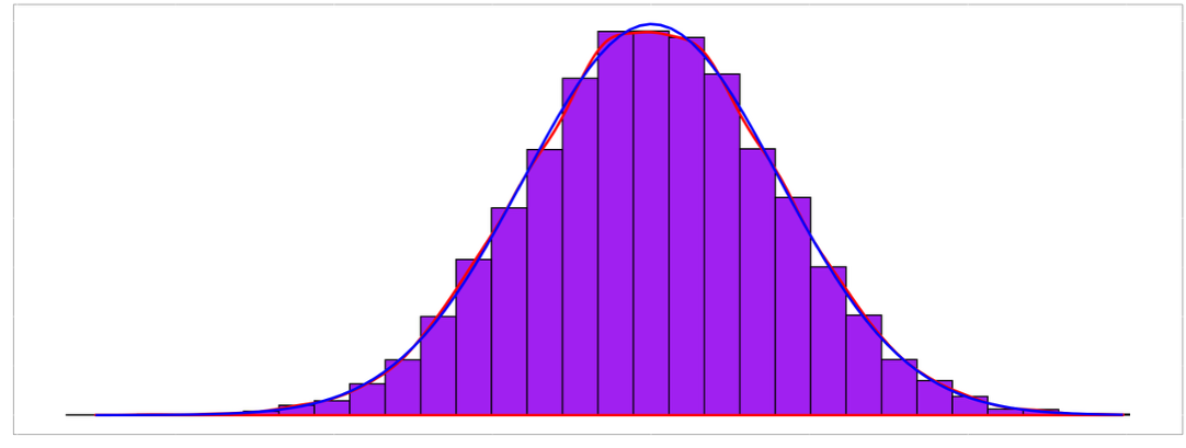
Fig. 6.32 Comparing actual data distribution (purple histogram) with its smooth estimate (red) and fitted normal curve (blue)*

When data follows a normal distribution, these three elements align closely. Deviations reveal specific patterns:

• Skewness: The red curve shifts away from the blue curve

• Heavy tails: The red curve extends further than the blue curve

• Light tails: The red curve falls short of the blue curve’s extent

• Multimodality: The red curve shows multiple peaks while the blue curve shows only one

B. Normal Probability Plots: A Sophisticated Diagnostic

Normal probability plots (also called QQ-plots for “quantile-quantile plots”) provide a more sensitive method for detecting departures from normality. These plots directly compare the quantiles of our data with the quantiles we would expect if the data truly came from a normal distribution.

Steps of Constructing a QQ-Plot

1. Order the Data

   Arrange the \(n\) observations from smallest to largest: \(x_{(1)} \leq x_{(2)} \leq \cdots \leq x_{(n)}\).

2. Assign Theoretical Probabilities

   Each ordered observation \(x_{(i)}\) represents approximately the \(\frac{i-0.5}{n}\) quantile of the data distribution. The adjustment of \(-0.5\) centers each data point within its expected quantile interval, providing more accurate comparisons.

3. Find Corresponding Normal Quantiles

   For each probability \(p_i = \frac{i-0.5}{n}\), find the z-value \(z_i\) such that \(\Phi(z_i) = p_i\). These are the theoretical quantiles we would expect if the data came from a standard normal distribution.

4. Create the Plot

   Plot the ordered data values \(x_{(i)}\) (y-axis) against the theoretical quantiles \(z_i\) (x-axis).

5. Add a Reference Line

   The reference line \(y = \bar{x} + s \cdot z\) shows where points would fall if the data perfectly matched a normal distribution with the sample’s mean and standard deviation.

Interpreting QQ-Plots

The power of QQ-plots lies in how different departures from normality create characteristic patterns.

Perfect Normality: Points fall exactly on the reference line.

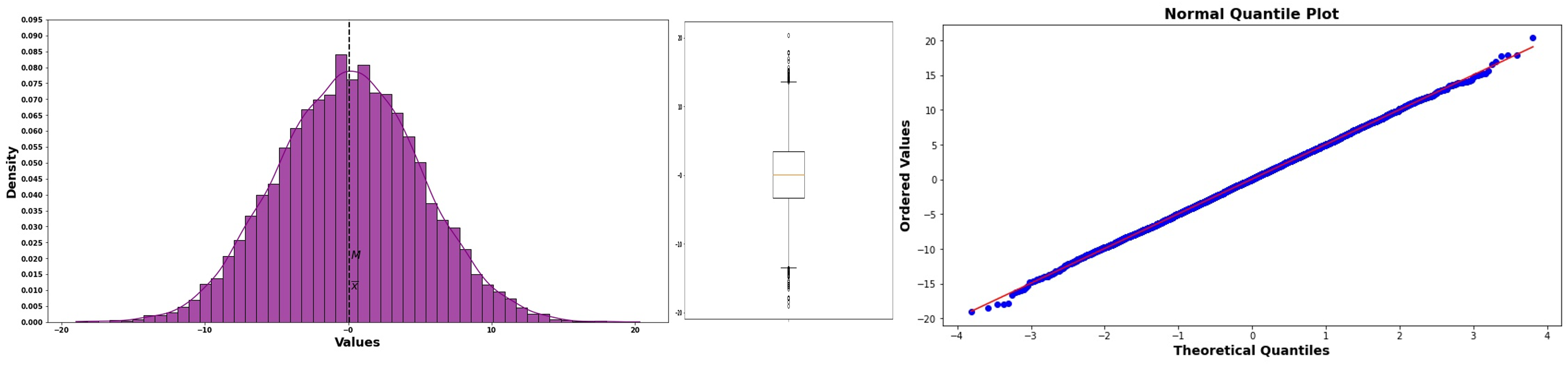
Fig. 6.33 Normal probability plot for normal data

Long Tails: Points begin below the line but curves above for larger values.

• Data has more extreme values than a normal distribution would predict

• The lower tail extends further left, upper tail extends further right

• Common in financial data, measurement errors with occasional large mistakes

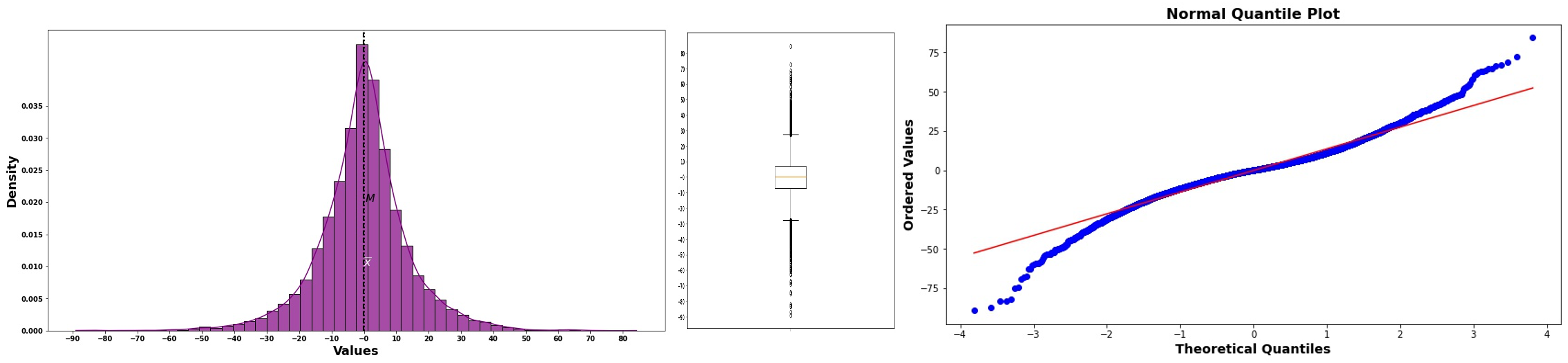
Fig. 6.34 Normal probability plot for long-tailed data

Short Tails: Points begin above the line but curves below for larger values.

• Data is more concentrated around the center than normal

• Fewer extreme values than expected

• Sometimes seen in truncated or bounded measurements

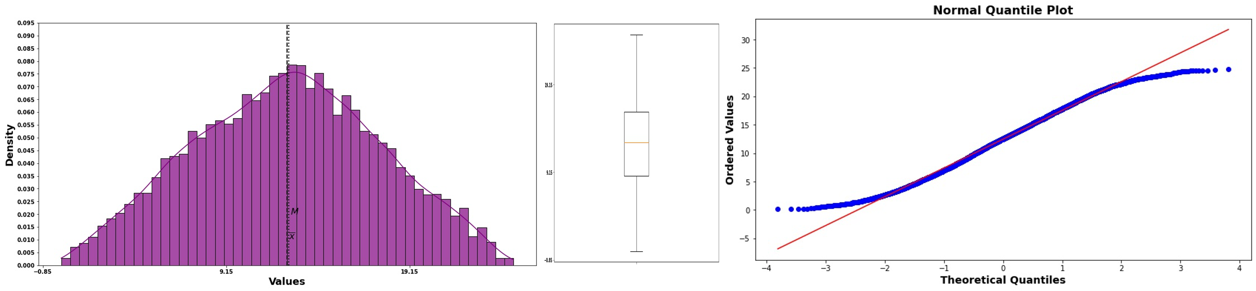
Fig. 6.35 Normal probability plot for short-tailed data

Right (Positive) Skewness: Concave-up curve

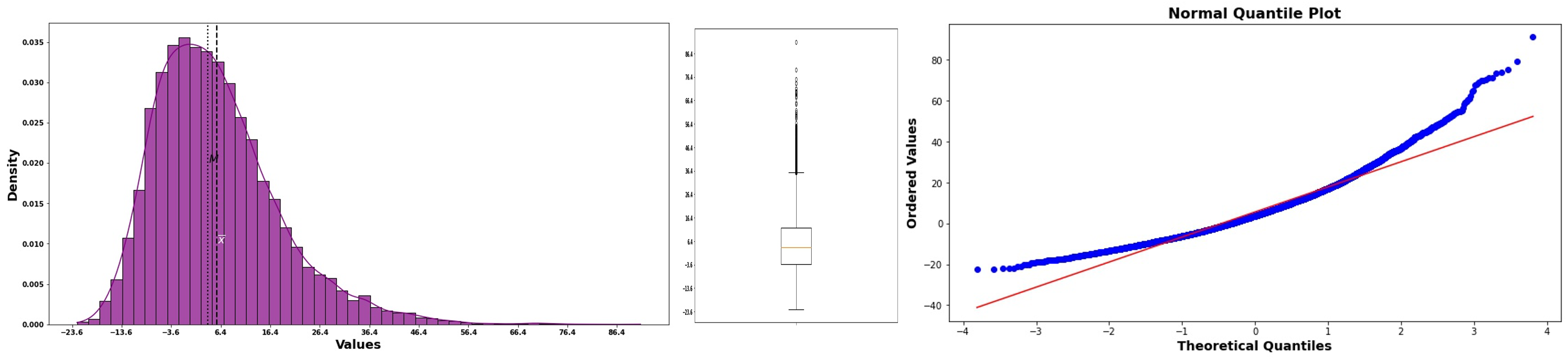
Fig. 6.36 Normal probability plot for right-skewed data

Left (Negative) Skewness: Concave-down curve

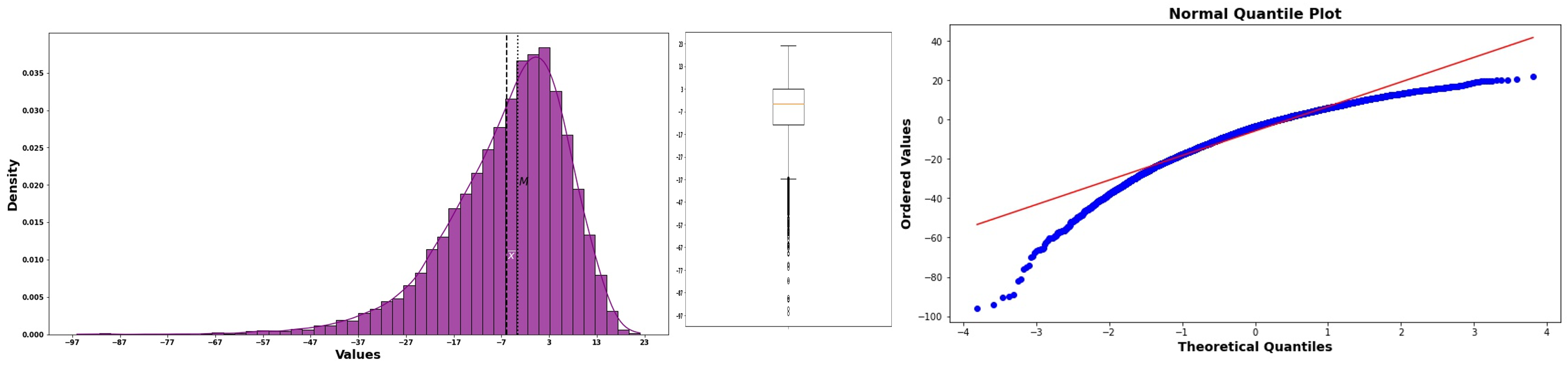
Fig. 6.37 Normal probability plot for left-skewed data

Bimodality: S-shaped curve with plateaus

• Points cluster in the middle region of the plot

• Suggests the data might come from a mixture of two populations

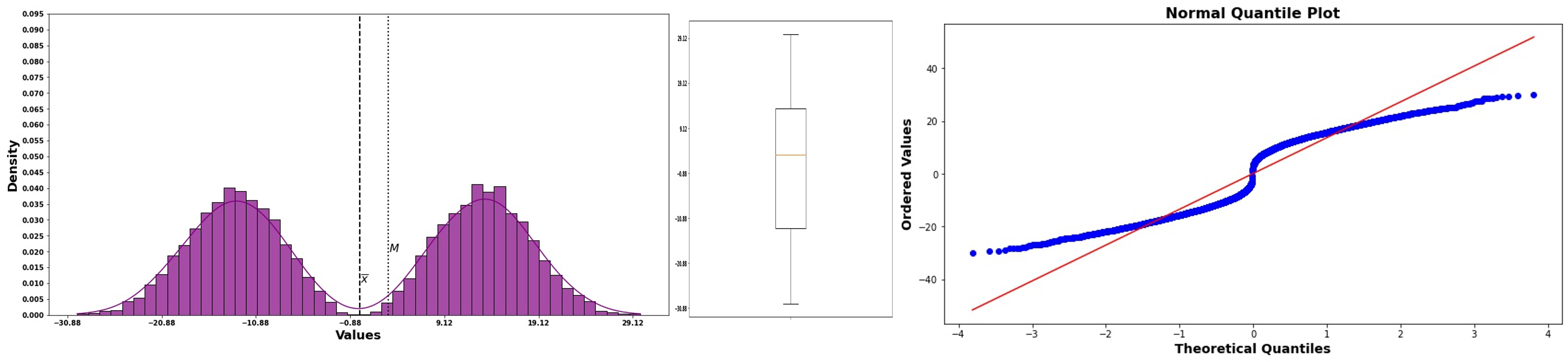
Fig. 6.38 Normal probability plot for bimodal data

6.4.10. Numerical Assessments for Normality

While visual methods provide intuitive insights, numerical methods offer precise, quantifiable assessments of normality.

A. The Empirical Rule in Reverse

Instead of using the 68-95-99.7 rule to predict probabilities, we can use it in reverse to check whether our data behaves as a normal distribution should:

For truly normal data,

• Approximately 68% of observations should fall within one standard deviation: \(\bar{x} \pm s\).

• Approximately 95% should fall within two standard deviations: \(\bar{x} \pm 2s\).

• Approximately 99.7% should fall within three standard deviations: \(\bar{x} \pm 3s\).

Implementation Steps

1. Calculate the sample mean \(\bar{x}\) and sample standard deviation \(s\).

2. Count observations within each interval.

3. Compare observed proportions to expected proportions (0.68, 0.95, 0.997).

4. Large deviations suggest non-normality.

B. The IQR-to-Standard Deviation Ratio

For normal distributions, there’s a consistent relationship between the interquartile range and the standard deviation. This relationship arises from the fixed positions of quantiles in any normal distribution.

For any normal distribution \(N(\mu, \sigma)\):

• The first quartile (25th percentile) occurs at \(\mu - 0.674\sigma\).

• The third quartile (75th percentile) occurs at \(\mu + 0.674\sigma\).

• Therefore: \(IQR = Q_3 - Q_1 = 1.348\sigma\).

• The ratio \(\frac{IQR}{\sigma} \approx 1.35\) (often rounded to 1.4).

Implementation Steps

1. Calculate the sample IQR and sample standard deviation \(s\).

2. Compute the ratio \(\frac{IQR}{s}\).

3. Values close to 1.35 suggest normality.

4. Values substantially different indicate departures from normality.

6.4.11. Formal Statistical Tests for Assessing Normality

While visual and numerical methods provide insights, formal statistical tests such as Shapiro-Wilk Test and Kolmovorov-Smirnov Tests offer rigorous hypothesis testing frameworks for normality. These tests are covered in more advanced statistics courses.

6.4.12. Bringing It All Together

Key Takeaways 📝

1. The normal distribution emerged from Gauss’s work on measurement errors and has become the most important continuous distribution in statistics.

2. The PDF \(f_X(x) = \frac{1}{\sqrt{2\pi \sigma}} e^{-\frac{1}{2}\left(\frac{x-\mu}{\sigma}\right)^2}\) is completely determined by two parameters: location \(\mu\) and scale \(\sigma\).

3. All normal distributions are symmetric, unimodal, and bell-shaped, with inflection points at \(\mu \pm \sigma\).

4. The empirical rule (68-95-99.7) provides quick probability estimates and applies to every normal distribution regardless of parameters.

5. Mathematical rigor: We proved the normal PDF is valid through polar coordinate integration and confirmed that \(E[X] = \mu\) and \(\text{Var}(X) = \sigma^2\).

6. The standard normal distribution \(N(0,1)\) serves as the foundation for all normal computations. The standardizing transformation \(Z = \frac{X-\mu}{\sigma}\) links any normal distribution to the standard one.

7. Assessing normality requires multiple approaches: visual methods (histograms, QQ-plots), numerical checks (empirical rule, IQR ratios), and formal tests (Shapiro-Wilk, Kolmogorov-Smirnov variants).

6.4.13. Exercises

These exercises develop your skills in working with normal distributions, including applying the empirical rule, standardization, computing probabilities (forward problems), finding percentiles (backward problems), and assessing normality.

Notation Convention

In this course, we write \(X \sim N(\mu, \sigma^2)\) where the second parameter is the variance. Always extract \(\sigma = \sqrt{\sigma^2}\) before standardizing. When using Z-tables, round z-scores to two decimal places. If a probability falls exactly between two table entries, average the corresponding z-values.

Exercise 1: Empirical Rule Applications

A semiconductor manufacturer produces microprocessors with clock speeds that follow a normal distribution with mean \(\mu = 3.2\) GHz and variance \(\sigma^2 = 0.0225\) GHz².

1. State the intervals containing approximately 68%, 95%, and 99.7% of clock speeds.

2. What percentage of processors have clock speeds between 2.9 GHz and 3.5 GHz?

3. A processor is considered “premium grade” if its clock speed exceeds 3.5 GHz. Approximately what percentage qualifies?

4. Quality control flags processors with clock speeds below 2.75 GHz as defective. Approximately what percentage is flagged?

Solution

Let \(X\) = clock speed (GHz), where \(X \sim N(\mu = 3.2, \sigma^2 = 0.0225)\).

First, extract the standard deviation: \(\sigma = \sqrt{0.0225} = 0.15\) GHz.

Part (a): Empirical rule intervals

• 68% interval: \(\mu \pm \sigma = 3.2 \pm 0.15 = (3.05, 3.35)\) GHz

• 95% interval: \(\mu \pm 2\sigma = 3.2 \pm 0.30 = (2.90, 3.50)\) GHz

• 99.7% interval: \(\mu \pm 3\sigma = 3.2 \pm 0.45 = (2.75, 3.65)\) GHz

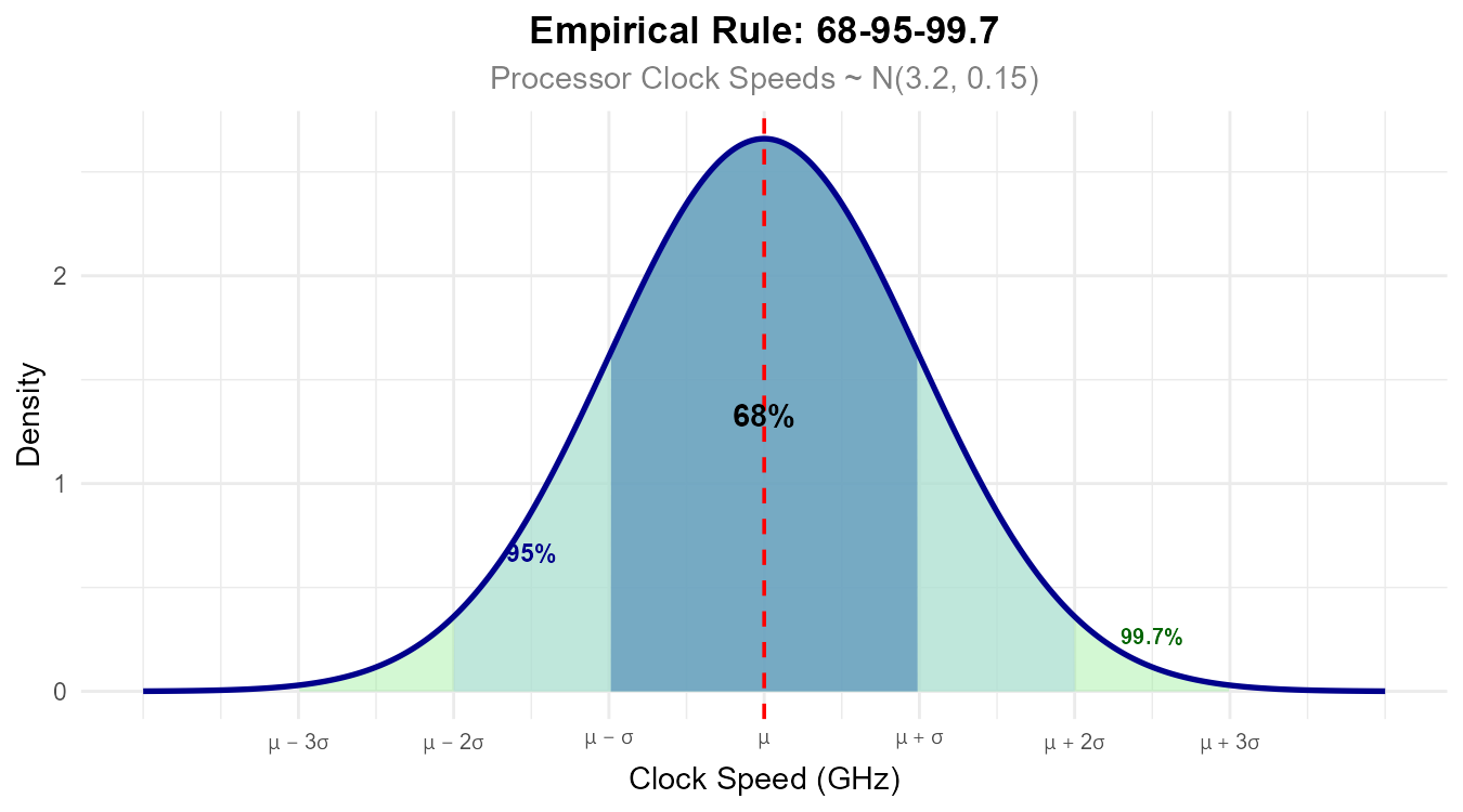
Fig. 6.39 The 68-95-99.7 rule applied to processor clock speeds.

Part (b): P(2.9 < X < 3.5)

Note that \(2.9 = \mu - 2\sigma\) and \(3.5 = \mu + 2\sigma\).

By the empirical rule, \(P(\mu - 2\sigma < X < \mu + 2\sigma) \approx 0.95\) or 95%.

Part (c): P(X > 3.5)

Since \(3.5 = \mu + 2\sigma\), we need \(P(X > \mu + 2\sigma)\).

From the empirical rule, 95% falls within \(\pm 2\sigma\), leaving 5% in both tails combined.

By symmetry, \(P(X > \mu + 2\sigma) \approx \frac{0.05}{2} = 0.025\) or 2.5%.

Part (d): P(X < 2.75)

Since \(2.75 = \mu - 3\sigma\), we need \(P(X < \mu - 3\sigma)\).

From the empirical rule, 99.7% falls within \(\pm 3\sigma\), leaving 0.3% in both tails.

By symmetry, \(P(X < \mu - 3\sigma) \approx \frac{0.003}{2} = 0.0015\) or 0.15%.

---

Exercise 2: Standardization and Z-Scores

The tensile strength of a carbon fiber composite follows a normal distribution with \(\mu = 600\) MPa and \(\sigma^2 = 1600\) MPa².

1. Find the z-score for a specimen with tensile strength 680 MPa. Interpret this value.

2. Find the z-score for a specimen with tensile strength 520 MPa. Interpret this value.

3. A specimen has a z-score of -0.75. What is its tensile strength?

4. Which is more unusual: a specimen with strength 700 MPa or one with strength 500 MPa? Justify using z-scores.

5. The specification requires tensile strength within 2 standard deviations of the mean. Express this requirement in terms of the original units (MPa).

Solution

Let \(X\) = tensile strength (MPa), where \(X \sim N(\mu = 600, \sigma^2 = 1600)\).

First, extract the standard deviation: \(\sigma = \sqrt{1600} = 40\) MPa.

Part (a): Z-score for x = 680

\[z = \frac{x - \mu}{\sigma} = \frac{680 - 600}{40} = \frac{80}{40} = 2.0\]

Interpretation: A tensile strength of 680 MPa is 2 standard deviations above the mean. This is an unusually high value—only about 2.5% of specimens exceed this strength.

Part (b): Z-score for x = 520

\[z = \frac{520 - 600}{40} = \frac{-80}{40} = -2.0\]

Interpretation: A tensile strength of 520 MPa is 2 standard deviations below the mean. This is an unusually low value.

Part (c): Tensile strength for z = -0.75

Solve for \(x\): \(x = \mu + z\sigma = 600 + (-0.75)(40) = 600 - 30 = 570\) MPa.

Part (d): Compare unusualness

For \(x = 700\): \(z = \frac{700 - 600}{40} = 2.5\)

For \(x = 500\): \(z = \frac{500 - 600}{40} = -2.5\)

Both have \(|z| = 2.5\), so they are equally unusual—each is 2.5 standard deviations from the mean.

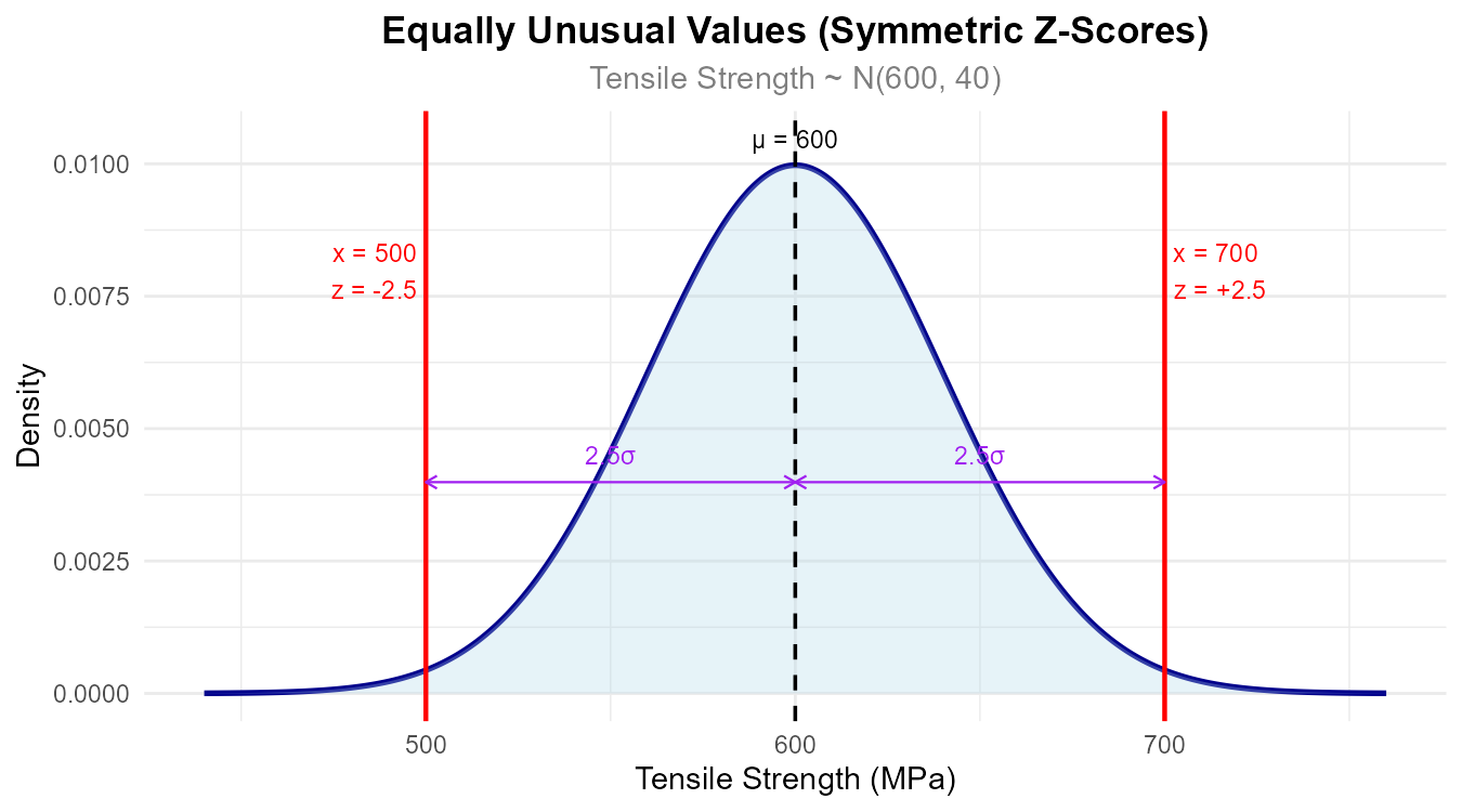
Fig. 6.40 Both values are equally far from the mean in terms of standard deviations.

Part (e): Specification in original units

Within 2 standard deviations: \(\mu \pm 2\sigma = 600 \pm 80 = (520, 680)\) MPa.

The specification requires tensile strength between 520 and 680 MPa.

---

Exercise 3: Forward Problem — Computing Probabilities

Response times for a web application follow a normal distribution with mean \(\mu = 250\) ms and variance \(\sigma^2 = 1225\) ms².

1. Find the probability that a randomly selected response takes less than 200 ms.

2. Find the probability that a response takes more than 300 ms.

3. Find the probability that a response takes between 220 and 280 ms.

4. The service level agreement (SLA) specifies that responses exceeding 320 ms are unacceptable. What proportion of responses violate the SLA?

Solution

Let \(X\) = response time (ms), where \(X \sim N(\mu = 250, \sigma^2 = 1225)\).

First, extract the standard deviation: \(\sigma = \sqrt{1225} = 35\) ms.

Part (a): P(X < 200)

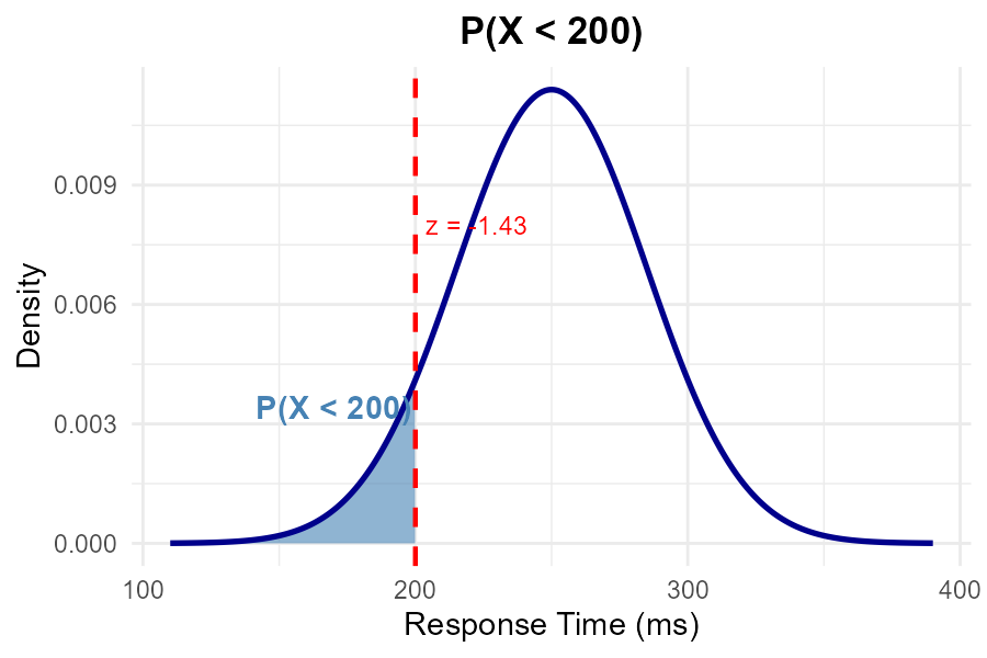
Fig. 6.41 Shaded region represents P(X < 200).

Step 1: Standardize.

\[z = \frac{200 - 250}{35} = \frac{-50}{35} = -1.43\]

Step 2: Use Z-table.

\[P(X < 200) = P(Z < -1.43) = \Phi(-1.43) = 0.0764\]

Part (b): P(X > 300)

Step 1: Standardize.

\[z = \frac{300 - 250}{35} = \frac{50}{35} = 1.43\]

Step 2: Use complement rule.

\[P(X > 300) = P(Z > 1.43) = 1 - \Phi(1.43) = 1 - 0.9236 = 0.0764\]

Note: By symmetry, P(X < 200) = P(X > 300) since both are 1.43 standard deviations from the mean.

Part (c): P(220 < X < 280)

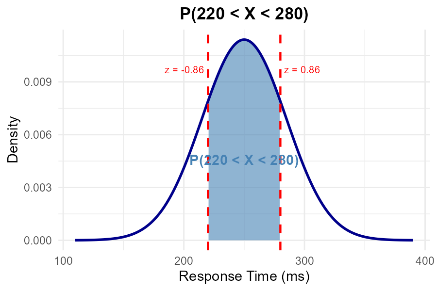
Fig. 6.42 Shaded region represents P(220 < X < 280).

Step 1: Standardize both bounds.

\[z_1 = \frac{220 - 250}{35} = -0.86 \quad \text{and} \quad z_2 = \frac{280 - 250}{35} = 0.86\]

Step 2: Use interval formula.

\[P(220 < X < 280) = \Phi(0.86) - \Phi(-0.86)\]

Step 3: Apply symmetry: \(\Phi(-0.86) = 1 - \Phi(0.86)\).

\[P(220 < X < 280) = \Phi(0.86) - (1 - \Phi(0.86)) = 2\Phi(0.86) - 1\]

Step 4: Look up and compute.

\[P(220 < X < 280) = 2(0.8051) - 1 = 0.6102\]

Part (d): P(X > 320)

Step 1: Standardize.

\[z = \frac{320 - 250}{35} = 2.0\]

Step 2: Compute.

\[P(X > 320) = 1 - \Phi(2.0) = 1 - 0.9772 = 0.0228\]

Approximately 2.28% of responses violate the SLA.

---

Exercise 4: Backward Problem — Finding Percentiles

The fuel efficiency of a hybrid vehicle model follows a normal distribution with mean \(\mu = 52\) mpg and variance \(\sigma^2 = 16\) mpg².

1. Find the 90th percentile of fuel efficiency.

2. Find the fuel efficiency value such that only 5% of vehicles perform worse (lower mpg).

3. Find the cutoffs for the middle 80% of fuel efficiency values.

4. A vehicle is classified as “high efficiency” if it ranks in the top 10%. What is the minimum fuel efficiency for this classification?

Solution

Let \(X\) = fuel efficiency (mpg), where \(X \sim N(\mu = 52, \sigma^2 = 16)\).

First, extract the standard deviation: \(\sigma = \sqrt{16} = 4\) mpg.

Part (a): 90th percentile

We seek \(x_{0.90}\) such that \(P(X \leq x_{0.90}) = 0.90\).

Step 1: Find \(z_{0.90}\) from Z-table by locating 0.90 in the body.

From the table: \(\Phi(1.28) = 0.8997\) and \(\Phi(1.29) = 0.9015\).

Since \(|0.90 - 0.8997| = 0.0003 < |0.90 - 0.9015| = 0.0015\), we use \(z_{0.90} = 1.28\).

Step 2: Convert to original scale.

\[x_{0.90} = \mu + z_{0.90} \cdot \sigma = 52 + 1.28(4) = 52 + 5.12 = 57.12 \text{ mpg}\]

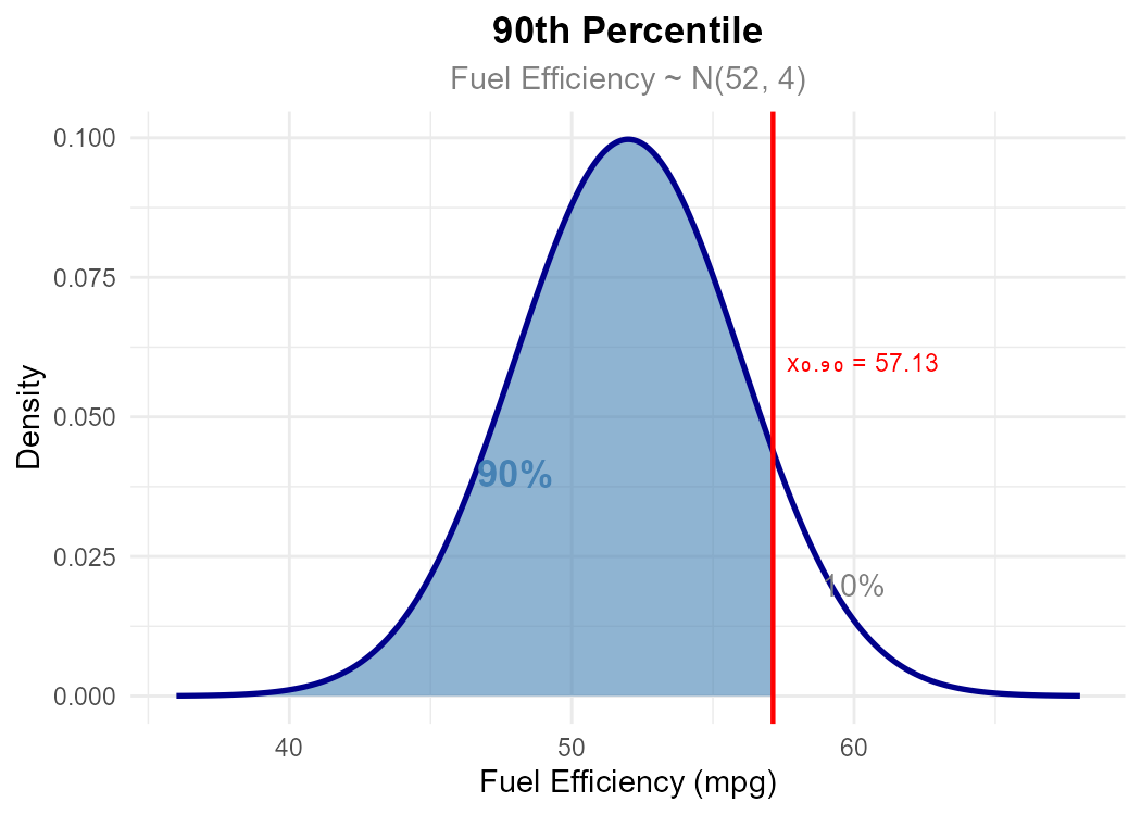
Fig. 6.43 The 90th percentile: 90% of vehicles have fuel efficiency at or below 57.12 mpg.

Part (b): 5th percentile

We seek \(x_{0.05}\) such that \(P(X \leq x_{0.05}) = 0.05\).

Step 1: Find \(z_{0.05}\) from the Z-table.

From the table: \(\Phi(-1.64) = 0.0505\) and \(\Phi(-1.65) = 0.0495\).

Since 0.05 is exactly halfway between 0.0495 and 0.0505, we average the z-values:

\[z_{0.05} = \frac{-1.64 + (-1.65)}{2} = -1.645\]

Step 2: Convert.

\[x_{0.05} = 52 + (-1.645)(4) = 52 - 6.58 = 45.42 \text{ mpg}\]

Only 5% of vehicles have fuel efficiency below 45.42 mpg.

Part (c): Middle 80% cutoffs

The middle 80% leaves 10% in each tail, so we need \(x_{0.10}\) and \(x_{0.90}\).

For the 10th percentile:

From the table: \(\Phi(-1.28) = 0.1003 \approx 0.10\), so \(z_{0.10} = -1.28\).

\(x_{0.10} = 52 + (-1.28)(4) = 46.88\) mpg

For the 90th percentile: \(z_{0.90} = 1.28\) (from part a).

\(x_{0.90} = 57.12\) mpg

The middle 80% falls between 46.88 and 57.12 mpg.

Part (d): Top 10% cutoff

“Top 10%” means \(P(X > x) = 0.10\), which is equivalent to \(P(X \leq x) = 0.90\).

This is the 90th percentile: 57.12 mpg (same as part a).

---

Exercise 5: Combined Forward and Backward Problems

Battery life for a laptop model follows a normal distribution with mean \(\mu = 8.5\) hours and variance \(\sigma^2 = 1.44\) hours².

1. What proportion of laptops have battery life between 7 and 10 hours?

2. The manufacturer wants to advertise a “minimum guaranteed battery life” that 95% of laptops will meet or exceed. What value should they advertise?

3. If 1000 laptops are sold, approximately how many will have battery life exceeding 11 hours?

4. A laptop’s battery life is at the 70th percentile. How many hours does it last?

5. Two laptops have battery lives of 6.5 hours and 10.5 hours. Which is more unusual relative to the distribution?

Solution

Let \(X\) = battery life (hours), where \(X \sim N(\mu = 8.5, \sigma^2 = 1.44)\).

First, extract the standard deviation: \(\sigma = \sqrt{1.44} = 1.2\) hours.

Part (a): P(7 < X < 10) — Forward problem

Standardize: \(z_1 = \frac{7 - 8.5}{1.2} = -1.25\) and \(z_2 = \frac{10 - 8.5}{1.2} = 1.25\).

From the Z-table: \(\Phi(1.25) = 0.8944\) and \(\Phi(-1.25) = 0.1056\).

\[P(7 < X < 10) = \Phi(1.25) - \Phi(-1.25) = 0.8944 - 0.1056 = 0.7888\]

Approximately 78.88% of laptops have battery life between 7 and 10 hours.

Part (b): 5th percentile — Backward problem

We need \(x_{0.05}\) such that 95% exceed this value (i.e., 5% fall below).

From the Z-table: \(\Phi(-1.64) = 0.0505\) and \(\Phi(-1.65) = 0.0495\).

Since 0.05 is exactly halfway, we average: \(z_{0.05} = \frac{-1.64 + (-1.65)}{2} = -1.645\).

\[x_{0.05} = 8.5 + (-1.645)(1.2) = 8.5 - 1.974 = 6.526 \text{ hours}\]

Under the model, exactly 95% of laptops exceed 6.53 hours. For a conservative marketing claim, the manufacturer should advertise 6.5 hours (rounded down to ensure the guarantee is met).

Part (c): Number exceeding 11 hours — Forward problem with application

Standardize: \(z = \frac{11 - 8.5}{1.2} = 2.08\).

\[P(X > 11) = 1 - \Phi(2.08) = 1 - 0.9812 = 0.0188\]

Expected number: \(1000 \times 0.0188 \approx 19\) laptops.

Part (d): 70th percentile — Backward problem

From the Z-table, we locate 0.70 in the body: \(\Phi(0.52) = 0.6985\) and \(\Phi(0.53) = 0.7019\).

Since \(|0.70 - 0.6985| = 0.0015 < |0.70 - 0.7019| = 0.0019\), we use \(z_{0.70} = 0.52\).

\[x_{0.70} = 8.5 + 0.52(1.2) = 8.5 + 0.624 = 9.12 \text{ hours}\]

Part (e): Compare unusualness

For \(x = 6.5\): \(z = \frac{6.5 - 8.5}{1.2} = -1.67\)

For \(x = 10.5\): \(z = \frac{10.5 - 8.5}{1.2} = 1.67\)

Both have \(|z| = 1.67\), so they are equally unusual.

---

Exercise 6: Parameter Identification

A normal distribution has specific characteristics. Use these to find the parameters \(\mu\) and \(\sigma\).

1. The inflection points of the PDF occur at \(x = 42\) and \(x = 58\). Find \(\mu\) and \(\sigma\).

2. The 16th percentile is 28 and the 84th percentile is 52. Find \(\mu\) and \(\sigma\).

3. The distribution has \(P(X < 70) = 0.90\) and \(P(X < 40) = 0.20\). Find \(\mu\) and \(\sigma\).

Solution

Part (a): Using inflection points

The inflection points of a normal PDF occur at \(\mu - \sigma\) and \(\mu + \sigma\).

\[\mu - \sigma = 42 \quad \text{and} \quad \mu + \sigma = 58\]

Adding: \(2\mu = 100 \implies \mu = 50\)

Subtracting: \(2\sigma = 16 \implies \sigma = 8\)

Answer: \(\mu = 50\), \(\sigma = 8\).

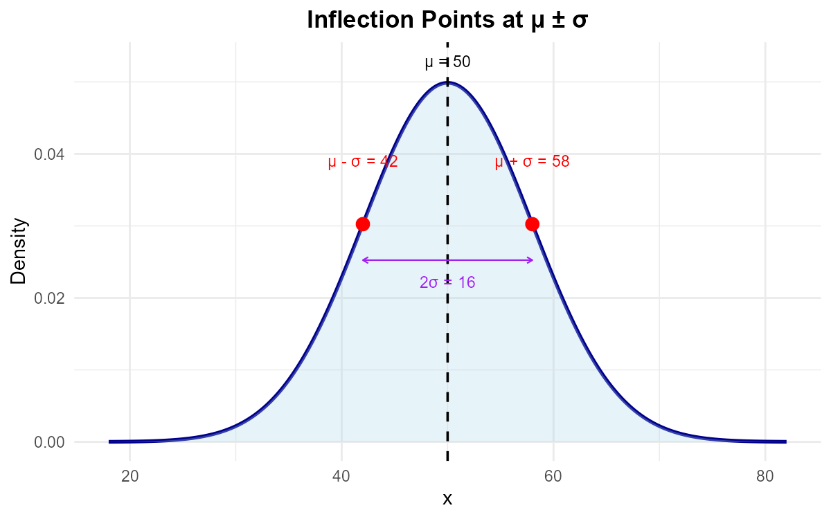
Fig. 6.44 Inflection points occur exactly at μ ± σ.

Part (b): Using symmetric percentiles

Note that the 16th and 84th percentiles are symmetric about the mean.

From the Z-table: \(\Phi(-0.99) = 0.1611\) and \(\Phi(-1.00) = 0.1587\).

Since \(|0.16 - 0.1611| = 0.0011 < |0.16 - 0.1587| = 0.0013\), we use \(z_{0.16} = -0.99\).

By symmetry, \(z_{0.84} = 0.99\).

This gives us:

\[\mu - 0.99\sigma = 28 \quad \text{and} \quad \mu + 0.99\sigma = 52\]

Adding: \(2\mu = 80 \implies \mu = 40\)

Subtracting: \(1.98\sigma = 24 \implies \sigma = 12.12\)

Answer: \(\mu = 40\), \(\sigma \approx 12.1\) (or \(\sigma^2 \approx 147\)).

Part (c): Using two probability statements

From \(P(X < 70) = 0.90\): Looking up 0.90 in the Z-table, \(\Phi(1.28) = 0.8997 \approx 0.90\), so \(z = 1.28\).

From \(P(X < 40) = 0.20\): Looking up 0.20, \(\Phi(-0.84) = 0.2005 \approx 0.20\), so \(z = -0.84\).

Setting up equations:

\[\frac{70 - \mu}{\sigma} = 1.28 \implies 70 - \mu = 1.28\sigma\]

\[\frac{40 - \mu}{\sigma} = -0.84 \implies 40 - \mu = -0.84\sigma\]

Subtracting the second from the first:

\[30 = 1.28\sigma + 0.84\sigma = 2.12\sigma \implies \sigma = \frac{30}{2.12} = 14.15\]

Substituting back: \(\mu = 70 - 1.28(14.15) = 70 - 18.11 = 51.89\)

Answer: \(\mu \approx 51.9\), \(\sigma \approx 14.2\) (or \(\sigma^2 \approx 200\)).

---

Exercise 7: Assessing Normality — Visual Methods

A materials engineer collects 50 measurements of yield strength (MPa) for aluminum alloy specimens. The sample statistics are \(\bar{x} = 275.3\) MPa and \(s = 12.8\) MPa.

The histogram and QQ-plot are shown below.

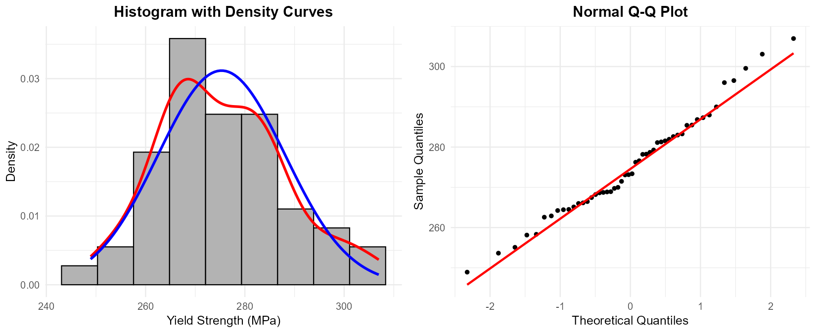
Fig. 6.45 Left: Histogram with kernel density (red) and normal curve (blue). Right: Normal QQ-plot.

1. Based on the histogram, does the data appear approximately normal? Comment on the alignment of the kernel density curve and the fitted normal curve.

2. Interpret the QQ-plot. Do the points follow the reference line reasonably well?

3. Identify any specific departures from normality visible in either plot.

4. Overall, would you conclude the normality assumption is reasonable for this data?

Solution

Part (a): Histogram interpretation

The histogram shows a roughly symmetric, unimodal distribution. The kernel density curve (red) and fitted normal curve (blue) align reasonably well, with both showing a bell-shaped pattern centered near 275 MPa. There is some minor roughness in the kernel density due to sampling variation with n=50, but no obvious skewness (neither tail appears systematically longer than the other).

Part (b): QQ-plot interpretation

The QQ-plot shows points that generally follow the reference line from the lower-left to upper-right. Most points fall close to or on the line, suggesting the data quantiles match the theoretical normal quantiles well. There is no systematic curvature (which would indicate skewness) or S-shape (which would indicate heavy/light tails).

Part (c): Specific departures

Examining the plots for specific features:

• Skewness: No evidence—both tails appear similar in length.

• Outliers: No points in the QQ-plot are dramatically far from the line.

• Tail behavior: The extreme points in the QQ-plot do not show systematic curvature at either end.

Minor deviations are expected with n=50 due to sampling variability.

Part (d): Conclusion

Based on both visual assessments, the normality assumption appears reasonable for this data. The histogram is approximately symmetric and bell-shaped, and the QQ-plot shows points close to the reference line with no systematic patterns of departure.

---

Exercise 8: Assessing Normality — Numerical Methods

For the aluminum alloy data from Exercise 7 (\(n = 50\), \(\bar{x} = 275.3\) MPa, \(s = 12.8\) MPa), additional sample statistics are provided:

• Sample IQR: 17.1 MPa

• Observations within \(\bar{x} \pm s\): 34 out of 50

• Observations within \(\bar{x} \pm 2s\): 48 out of 50

• Observations within \(\bar{x} \pm 3s\): 50 out of 50

1. Apply the empirical rule check. Compare the observed proportions to the expected 68-95-99.7 values.

2. Compute the IQR-to-standard deviation ratio. Compare to the theoretical value for normal distributions.

3. Based on these numerical checks, does the data appear consistent with a normal distribution?

Solution

Part (a): Empirical rule check

Interval	Observed Count	Observed %	Expected %	Difference
\(\bar{x} \pm 1s\)	34/50	68%	68%	0%
\(\bar{x} \pm 2s\)	48/50	96%	95%	+1%
\(\bar{x} \pm 3s\)	50/50	100%	99.7%	+0.3%

The observed proportions are remarkably close to the expected values.

Note on sampling variability: With n=50 observations from a true normal distribution, the count within \(\pm 2\sigma\) follows approximately a Binomial(50, 0.95) distribution. The standard deviation of this count is \(\sqrt{50 \times 0.95 \times 0.05} \approx 1.5\), so observing 48 instead of the expected 47.5 is well within normal sampling variation.

Part (b): IQR-to-SD ratio

\[\frac{\text{IQR}}{s} = \frac{17.1}{12.8} = 1.336\]

For a normal distribution, the theoretical ratio is approximately 1.35.

The observed ratio (1.336) is very close to the expected value, indicating consistency with normality.

Part (c): Conclusion

Yes, the numerical checks strongly support normality:

• Empirical rule proportions match almost exactly (68%, 96%, 100% vs. 68%, 95%, 99.7%)

• IQR/SD ratio (1.336) is very close to the theoretical 1.35

Combined with the visual assessments from Exercise 7, we have strong evidence that the normality assumption is appropriate.

---

Exercise 9: Identifying Non-Normal Distributions

Four datasets have been analyzed with QQ-plots shown below. Match each QQ-plot pattern to the appropriate description of the underlying distribution.

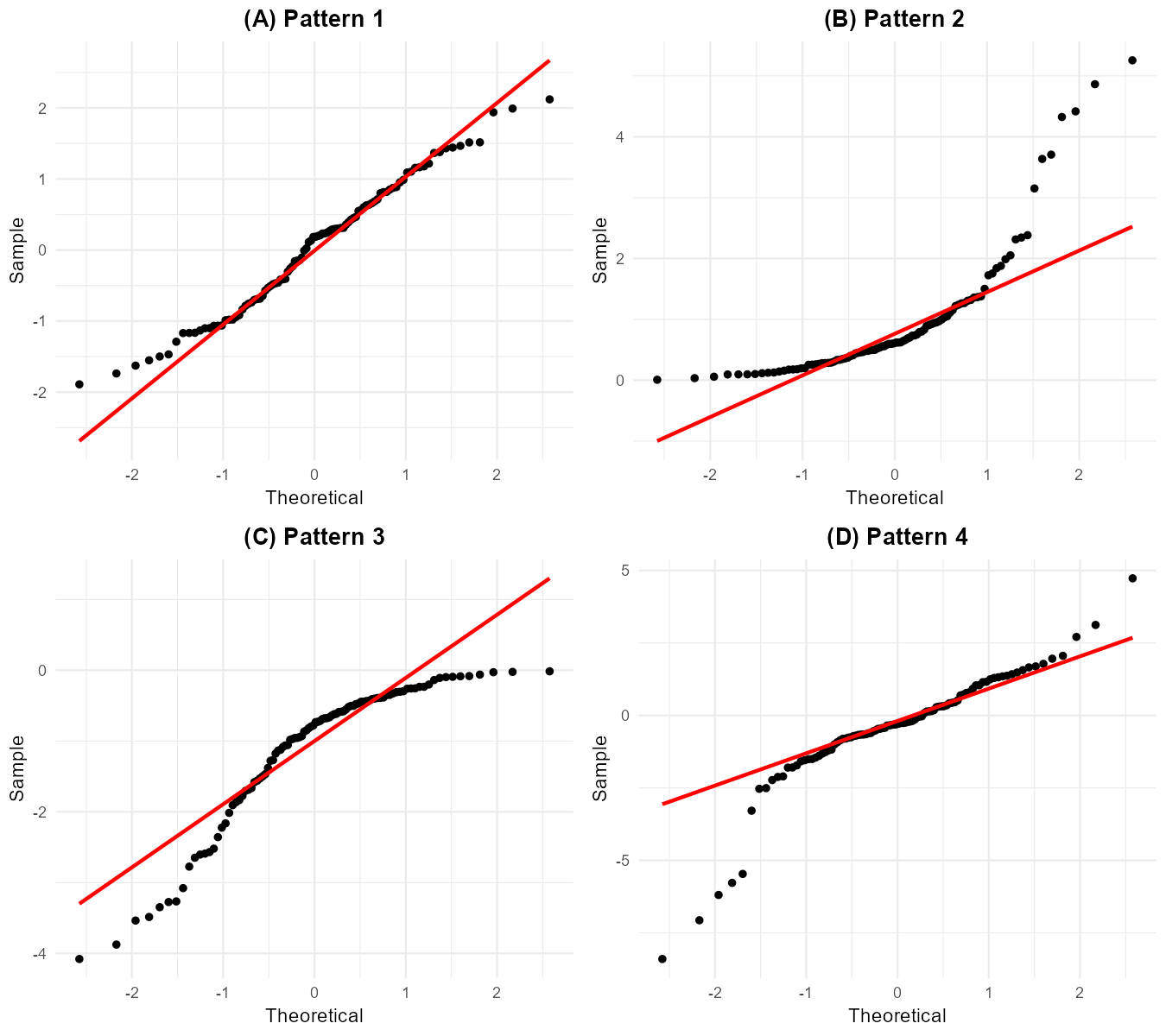
Fig. 6.46 Four QQ-plots: (A) upper-left, (B) upper-right, (C) lower-left, (D) lower-right.

Match each plot (A, B, C, D) with one of these descriptions:

1. Right-skewed distribution (long right tail)

2. Left-skewed distribution (long left tail)

3. Heavy-tailed distribution (more extreme values than normal)

4. Approximately normal distribution

Solution

Plot A: Approximately normal distribution (Description 4)

The points fall close to the reference line throughout, indicating the sample quantiles match the theoretical normal quantiles well.

Plot B: Right-skewed distribution (Description 1)

The points curve upward (concave up) away from the reference line. This indicates:

• Lower quantiles match well

• Upper quantiles are larger than expected for a normal

• The right tail is stretched out (right/positive skew)

Plot C: Left-skewed distribution (Description 2)

The points curve downward (concave down) away from the reference line. This indicates:

• Lower quantiles are smaller than expected

• Upper quantiles match reasonably

• The left tail is stretched out (left/negative skew)

Plot D: Heavy-tailed distribution (Description 3)

The points form an S-shape:

• Lower quantiles fall below the line (more extreme negative values than normal)

• Upper quantiles rise above the line (more extreme positive values than normal)

• Both tails are heavier than a normal distribution

Summary Table:

Plot	Pattern	Distribution Type
A	Points on line	Normal
B	Concave up (curved up)	Right-skewed
C	Concave down (curved down)	Left-skewed
D	S-shaped	Heavy-tailed

---

6.4.14. Additional Practice Problems

True/False Questions (1 point each)

1. For any normal distribution, the mean equals the median.

   Ⓣ or Ⓕ

2. If \(X \sim N(100, 25)\), then the standard deviation is 5.

   Ⓣ or Ⓕ

3. A z-score of -1.5 indicates a value 1.5 standard deviations below the mean.

   Ⓣ or Ⓕ

4. For a standard normal distribution, \(P(Z > 0) = 0.5\).

   Ⓣ or Ⓕ

5. The inflection points of a normal PDF occur at \(\mu \pm 2\sigma\).

   Ⓣ or Ⓕ

6. If \(X \sim N(\mu, \sigma^2)\), then \(P(X < \mu) = 0.5\).

   Ⓣ or Ⓕ

7. A QQ-plot that curves upward indicates left-skewed data.

   Ⓣ or Ⓕ

8. For normal distributions, the IQR is approximately 1.35 times the standard deviation.

   Ⓣ or Ⓕ

Multiple Choice Questions (2 points each)

9. For \(X \sim N(50, 100)\), what is \(P(X < 60)\)?

   Ⓐ 0.6915

   Ⓑ 0.8413

   Ⓒ 0.9332

   Ⓓ 0.9772

10. If \(Z \sim N(0, 1)\) and \(P(Z < z) = 0.75\), what is \(z\)?

    Ⓐ 0.25

    Ⓑ 0.67

    Ⓒ 0.75

    Ⓓ 1.15

11. A normal distribution has \(\mu = 80\) and \(\sigma = 10\). What value has a z-score of -2?

    Ⓐ 60

    Ⓑ 70

    Ⓒ 78

    Ⓓ 100

12. According to the empirical rule, approximately what percentage of values fall more than 2 standard deviations from the mean?

    Ⓐ 2.5%

    Ⓑ 5%

    Ⓒ 32%

    Ⓓ 95%

13. For \(X \sim N(200, 400)\), what is the 95th percentile?

    Ⓐ 212.8

    Ⓑ 225.8

    Ⓒ 232.9

    Ⓓ 265.8

14. Which QQ-plot pattern indicates heavy tails?

    Ⓐ Points curve upward (concave up)

    Ⓑ Points curve downward (concave down)

    Ⓒ S-shaped pattern (low points below line, high points above)

    Ⓓ Points fall exactly on the reference line

Answers to Practice Problems

True/False Answers:

1. True — Normal distributions are perfectly symmetric, so mean = median.

2. True — In the notation \(N(\mu, \sigma^2)\), the second parameter is variance. Since \(\sigma^2 = 25\), we have \(\sigma = \sqrt{25} = 5\).

3. True — A z-score represents the number of standard deviations from the mean. Negative z-scores are below the mean.

4. True — By symmetry around 0, exactly half the probability is above 0 and half below.

5. False — Inflection points occur at \(\mu \pm \sigma\) (one standard deviation), not two.

6. True — By symmetry, exactly 50% of the distribution falls below the mean.

7. False — A QQ-plot that curves upward (concave up) indicates right-skewed data. Left-skewed data produces a concave-down pattern.

8. True — For normal distributions, IQR ≈ 1.35σ (specifically, 1.348σ).

Multiple Choice Answers:

9. Ⓑ — \(\sigma = \sqrt{100} = 10\), so \(z = \frac{60-50}{10} = 1.0\). From the table: \(\Phi(1.00) = 0.8413\).

10. Ⓑ — Looking up 0.75 in the Z-table body: \(\Phi(0.67) = 0.7486\) and \(\Phi(0.68) = 0.7517\). Since 0.7486 is closer to 0.75, \(z \approx 0.67\).

11. Ⓐ — \(x = \mu + z\sigma = 80 + (-2)(10) = 60\).

12. Ⓑ — 95% fall within ±2σ, so 5% fall outside (more than 2 SD from mean).

13. Ⓒ — \(\sigma = \sqrt{400} = 20\). For \(z_{0.95}\): \(\Phi(1.64) = 0.9495\) and \(\Phi(1.65) = 0.9505\). Since 0.95 is exactly halfway, \(z_{0.95} = 1.645\). Thus \(x_{0.95} = 200 + 1.645(20) = 232.9\).

14. Ⓒ — Heavy tails produce an S-shaped pattern where both extremes deviate from the line in opposite directions.