Slides 📊

Download Chapter 5 slides (PPTX)

5.7. The Poisson Distribution

While the binomial distribution helps us count successes in a fixed number of trials, many real-world situations involve counting rare events that occur randomly over time or space. Think about counting phone calls to a help desk during an hour, defects in a length of computer tape, or radioactive particles emitted by a radioactive substance. These scenarios share a structure that leads us to another fundamental distribution in statistics: the Poisson distribution.

Road Map 🧭

• Identify situations where the Poisson distribution applies.

• Master the Poisson probability mass function and its single parameter \(\lambda\).

• Derive the Poisson expected value and variance using infinite series techniques.

• Understand how the interval length affects the parameter \(\lambda\).

5.7.1. From Counting Events to Modeling Rates

The Poisson distribution emerges when we count events that occur randomly over continuous intervals of time, space, or volume. Unlike a binomial experiment which involves a fixed number of trials, the number of events in a Poisson process is theoretically unlimited.

What Makes a Process Poisson?

A Poisson process has three essential properties:

1. Stationary and Proportional

• The probability that an event occurs in any interval depends only on the length of that interval, not on where the interval occurs (stationarity).

• Equal-sized intervals have the same probability distribution, and longer intervals have proportionally higher probabilities of containing events.

For example, suppose we’re counting phone calls to a help desk that has a constant call rate. The probability of receiving exactly one call should be the same whether we look at 9-10 AM or 2-3 PM. Furthermore, if we expect 3 calls per hour on average, we should expect 6 calls per two-hour period.

2. Independent Events

Individual events occur independently of each other. The occurrence of one event doesn’t influence when the next event will happen. Additionally, the number of events in non-overlapping intervals are independent of each other.

In our phone call example, receiving three calls between 9-10 AM doesn’t affect the number of calls received between 10-11 AM.

3.Orderliness (no bunching)

Events cannot occur simultaneously. In sufficiently small intervals, the chance of two or more events occurring is negligible. Events effectively arrive one at a time.

Examples of Poisson Distributions

Several real-world scenarios approximately follow the rules of Poisson processes:

• Radioactive decay: The number of alpha particles emitted from uranium-238 in one minute

• Call centers: The number of calls received during busy hours on any given day

• Quality control: The number of flaws on a computer tape of fixed length

• Ecology: The number of dead trees in a square mile of forest

• Traffic: The number of accidents at an intersection per month

5.7.2. The Poisson Distribution

When events follow a Poisson process, we model the count of events using a Poisson distribution.

Definition

A Poisson random variable \(X\) counts the number of independently occurring events in a fixed interval, where events occur at some average rate \(\lambda\) (lambda) per interval.

When \(X\) has a Poisson distribution, we write \(X \sim \text{Poisson}(\lambda)\).

Probability Mass Function

The Poisson PMF gives the probability of observing exactly \(x\) events:

\[p_X(x) = \frac{e^{-\lambda} \lambda^x}{x!}\]

for \(x \in \text{supp}(X) = \{0, 1, 2, 3, ...\}\).

Notice several key features of this distribution:

• Single parameter: Unlike the binomial distribution which has two parameters (\(n\) and \(p\)), Poisson has only one parameter \(\lambda\).

• Unbounded support: A Poisson random variable can theoretically take any non-negative integer value, unlike binomial whose support is bounded above by \(n\).

5.7.3. Expected Value and Variance: The Power of \(\lambda\)

One of the most elegant features of the Poisson distribution is that its parameter \(\lambda\) completely determines both the center and spread of the distribution.

Expected Value

To find \(E[X]\) for a Poisson random variable, we use the definition of expected value:

\[E[X] = \sum_{x=0}^{\infty} x \cdot p_X(x) = \sum_{x=0}^{\infty} x \cdot \frac{e^{-\lambda} \lambda^x}{x!}\]

Since the first term equals zero with \(x = 0\), the summation effectively begins at \(x = 1\). Then in each term, we can cancel \(x\) with the \(x\) contained in \(x!\) of the denominator. Since \(e^\lambda\) does not depend on \(x\), we can bring this outside the summation:

\[E[X] = \sum_{x=1}^{\infty} x \cdot \frac{e^{-\lambda} \lambda^x}{x!} = e^{-\lambda} \sum_{x=1}^{\infty} \frac{\lambda^x}{(x-1)!}\]

Substituting \(u = x - 1\), we get:

\[E[X] = e^{-\lambda} \lambda \sum_{u=0}^{\infty} \frac{\lambda^u}{u!}\]

The sum is the Taylor series for \(e^λ\). Therefore:

\[E[X] = e^{-\lambda} \lambda \cdot e^{\lambda} = \lambda\]

Variance

For the variance, we use \(\text{Var}(X) = E[X^2] - (E[X])^2\). We already know \(E[X] = \lambda\), and we need \(E[X^2]\):

\[E[X^2] = \sum_{x=0}^{\infty} x^2 \cdot \frac{e^{-\lambda} \lambda^x}{x!}\]

Through similar algebraic manipulation (starting at \(x = 1\), canceling factorials, and using substitutions), we can show:

\[E[X^2] = \lambda^2 + \lambda\]

Therefore:

\[\text{Var}(X) = E[X^2] - (E[X])^2 = (\lambda^2 + \lambda) - \lambda^2 = \lambda\]

Summary of Poisson Distribution Properties

For \(X \sim Poisson(\lambda)\):

\[\begin{split}&\mu_X = E[X] = \lambda \\ &\sigma_X^2 = \text{Var}(X) = \lambda \\ &\sigma_X = \sqrt{\lambda}\end{split}\]

The summary reveals a remarkable property of Poisson distribution; knowing \(\lambda\) tells us everything about the distribution’s location and spread.

5.7.4. Visualizing Poisson Distributions

Small \(\lambda \, (\lambda=1)\)

When events are rare, most probability concentrates at 0 and 1, with a long right tail. The distribution is highly right-skewed.

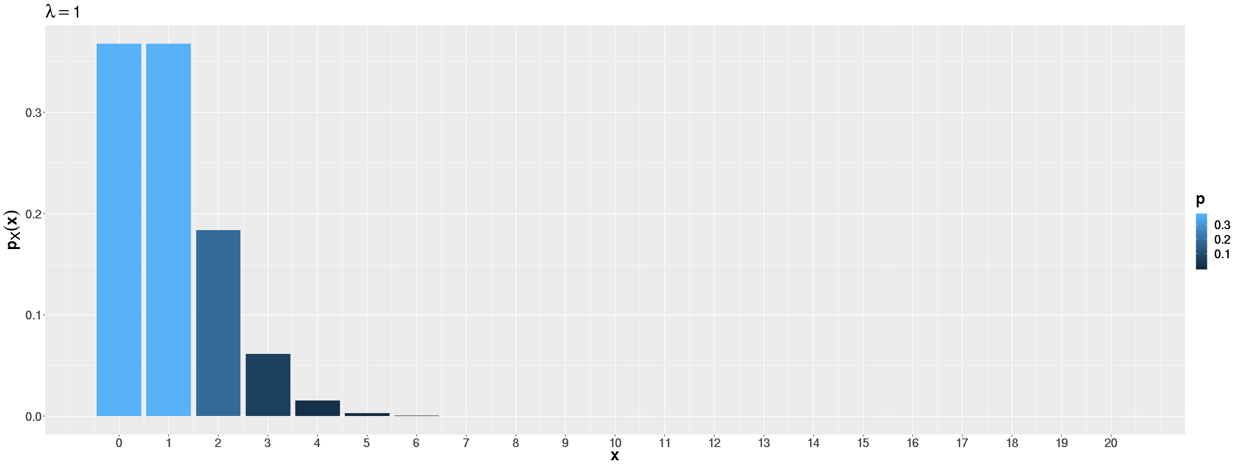
Fig. 5.11 \(\lambda=1\)

Moderate \(\lambda \, (\lambda=2.5)\)

As \(\lambda\) increases, the mode shifts right and the distribution becomes less skewed. More probability spreads across multiple values.

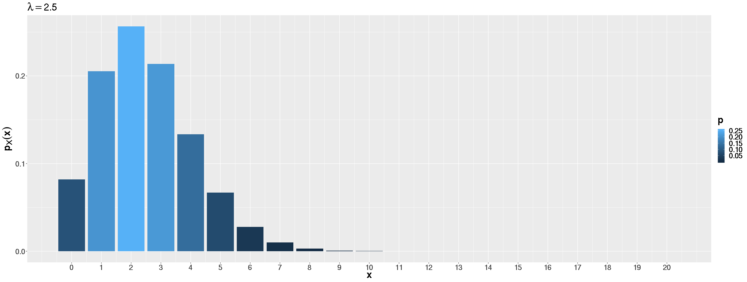
Fig. 5.12 \(\lambda=2.5\)

Large \(\lambda \, (\lambda=10)\)

For larger \(\lambda\) values, the distribution approaches a symmetric, bell-shaped curve centered around \(\lambda\). The resemblance to a normal distribution becomes quite strong.

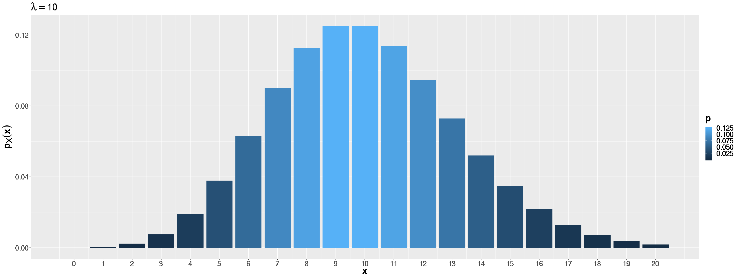
Fig. 5.13 \(\lambda=10\)

Example💡: IT Consultant Call Analysis

An IT consultant receives an average of 3 calls per hour. We want to model the number of calls using a Poisson distribution and answer several probability questions.

Setting Up the Model

Let \(X\) count number of calls the consultant receives in the next hour.

• Stationary and Proportional: Call rate is constant over time. ✓

• Independent: One call doesn’t influence when the next occurs. ✓

• Orderliness: Calls don’t occur simultaneously. ✓

Therefore: \(X \sim \text{Poisson}(\lambda = 3)\).

Solving Probability Problems

1. Find the probability of exactly one call.

   \[P(X = 1) = \frac{e^{-3} \cdot 3^1}{1!} = \frac{3e^{-3}}{1} ≈ 0.1494\]

2. Find the probability of more than one call. Using the complement rule:

   \[P(X > 1) = 1 - [P(X = 0) + P(X = 1)] = 1 - [e^{-3} + 3e^{-3}] ≈ 0.8009\]

3. Find the probability of exactly 5 calls in the next two hours.

   Since the rate is 3 calls per hour, over two hours we expect 2 × 3 = 6 calls on average. Let \(Y\) count the number of calls in the next two hours. Then \(Y \sim \text{Poisson}(\lambda = 6)\).

   \[P(Y = 5) = \frac{e^{-6} \cdot 6^5}{5!} ≈ 0.1606\]

4. Find the probability of 1 call in the next hour and 4 calls in the following hour.

   Let \(X_1\) count the calls in the first hour and \(X_2\) the calls in the second hour. Both have an average rate of 3, and since the two intervals are non-overlapping, \(X_1\) and \(X_2\) are indepdendent. This allows us to use the special multiplication rule:

   \[\begin{split}P(X_1=1 \cap X_2=4) &= P(X_1=1)P(X_2=4)\\ &=(0.8009)\left(\frac{e^{-3}3^4}{4!}\right) \\ &= (0.8009)(0.1680) \approx 0.1346\end{split}\]

5.7.5. When to Use Poisson vs. Binomial

Understanding when to use Poisson versus binomial distributions is crucial for proper statistical modeling.

Use Poisson When:

• Counting events over continuous intervals (time, space, volume).

• Events are rare relative to opportunity.

• The number of potential events is very large or unlimited.

• You know the average rate but not the total number of trials.

Use Binomial When:

• The number of independent trials is fixed.

• Each trial has exactly two outcomes.

• Probability of success is constant across trials.

• You’re counting successes among a known number of attempts.

Poisson as Binomial Approximation

Interestingly, Poisson can approximate binomial when \(n\) is large and \(p\) is small, with \(np \approx \lambda\). This connection highlights how these distributions relate to different aspects of the same underlying counting process.

5.7.6. Bringing It All Together

The Poisson distribution serves as a fundamental model for understanding random processes in fields ranging from telecommunications and quality control to epidemiology and reliability engineering. As we’ve seen, the key to successful application lies in recognizing when events satisfy the Poisson assumptions and correctly interpreting the rate parameter \(λ\) in context.

Key Takeaways 📝

1. The Poisson distribution models counts of rare events occurring over fixed intervals of time, space, or volume.

2. Three key properties that define Poisson processes are stationarity and proportional rates, independence of events, and unique event occurrences.

3. The PMF formula \(p_X(x) = \frac{e^{-\lambda}\lambda^x}{x!}\) applies to any non-negative interger \(x\).

4. The single parameter \(\lambda\) represents both the mean and variance: \(E[X] = \text{Var}(X) = λ\).

5. The shape of a Poisson distribution evolves from highly right-skewed to approximately symmetric as \(\lambda\) becomes larger.

Exercises

1. Identifying Poisson Processes: Determine whether each scenario could be modeled using a Poisson distribution. Explain your reasoning.

   1. The number of typos in a 10-page document

   2. The number of students who arrive late to a 50-student class

   3. The number of car accidents at a busy intersection per week

   4. The number of defective items in a batch of 100 manufactured products

2. Basic Probability Calculations: Emails arrive at a server at an average rate of 2.5 per minute. Assume this follows a Poisson distribution.

   1. What is the probability of receiving exactly 3 emails in the next minute?

   2. What is the probability of receiving no emails in the next minute?

   3. What is the probability of receiving more than 4 emails in the next minute?

   4. What are the mean and standard deviation for the number of emails per minute?

3. Parameter Scaling: A call center receives an average of 4 calls per hour during peak times.

   1. What is the probability of receiving exactly 2 calls in 30 minutes?

   2. What is the probability of receiving at least 10 calls in 3 hours?

   3. In how long an interval would you expect to receive exactly 1 call on average?