Slides 📊
6.1. Continuous Random Variables and Probability Density Functions
What happens when we want to model measurements rather than counts? How do we handle quantities like height, weight, temperature, or time—variables that can take on any value within a continuous range? This section explores the shift in mathematical framework that occurs when we move from the discrete world of “how many” to the continuous world of “how much.”
Road Map 🧭
Understand why continuous random variables require a different mathematical approach than discrete ones.
Define probability density functions (PDFs) as the continuous analog to probability mass functions.
Master the key concept that probabilities are areas under a PDF.
Learn the essential properties that make a function a valid PDF.
Find probabilities for continuous random variables by integrating the PDF.
6.1.1. Discrete vs. Continuous Random Variables
For random variables with a discrete support, we could assign positive probabilities to individual outcomes. It made perfect sense to say “the probability of getting exactly 3 heads in 10 coin flips is some specific value” because 3 was one of only eleven distinct outcomes (0 through 10 heads). Even when the support is countably infinite—as in the Poisson distribution—we could still assign probabilities in such a way that each value in the support had a positive probability (however small) while the total sum remains 1.
But many real-world phenomena involve measurements along a continuous scale, which has a vastly larger support than that of any discrete random variable. While we might record a person’s height as “5 feet 8 inches,” the actual height could be 5.75000… feet or 5.750001… feet. Between any two measurements, no matter how close, there are uncountably many possible intermediate values. If we tried to assign positive probabilities to each possible height—no matter how cleverly—we would end up with an infinite total, violating the fundamental requirement that all probabilities sum (or integrate) to 1.
The Resolution: Zero Probability for Any Single Point
We resolve this paradox by accepting that any single exact value has probability zero for continuous random variables. The probability that someone’s height is exactly 5.750000000… feet with infinite precision is zero, even though this height is perfectly possible.
This might seem counterintuitive at first. How can something be possible but have zero probability? Recall that probability can be seen as the relative size of an event compared to the whole. In the continuous case, we’re dealing with uncountably many possible values packed into any interval, so many that any single point is negligible in comparison. This makes the relative size, and thus the probability, of any one value equal to zero.
Then What Has a Positive Probability?
For continuous random variables, we discuss probabilities of intervals of values rather than single points. This aligns naturally with the graphical interpretation of probabilities as areas under a curve–regions with non-zero width will have a positive area, while a single point always has zero area.
6.1.2. Probability Density Functions: The Continuous Analog of Probability Mass Functions
From Histograms to Curves
Since we can’t assign probabilities to individual points, we need a different approach than PMF to describe the distribution of a continuous random variable. We can think of a continuous probability distribution as a curve that represents the limiting behavior of increasingly fine histograms for an increasingly large dataset.
In Fig. 6.1, the jagged histogram begins to approximate a curve as we collect more data and make the bins narrower. In the limit—with infinite data and infinitesimally narrow bins—we get a probability density function.
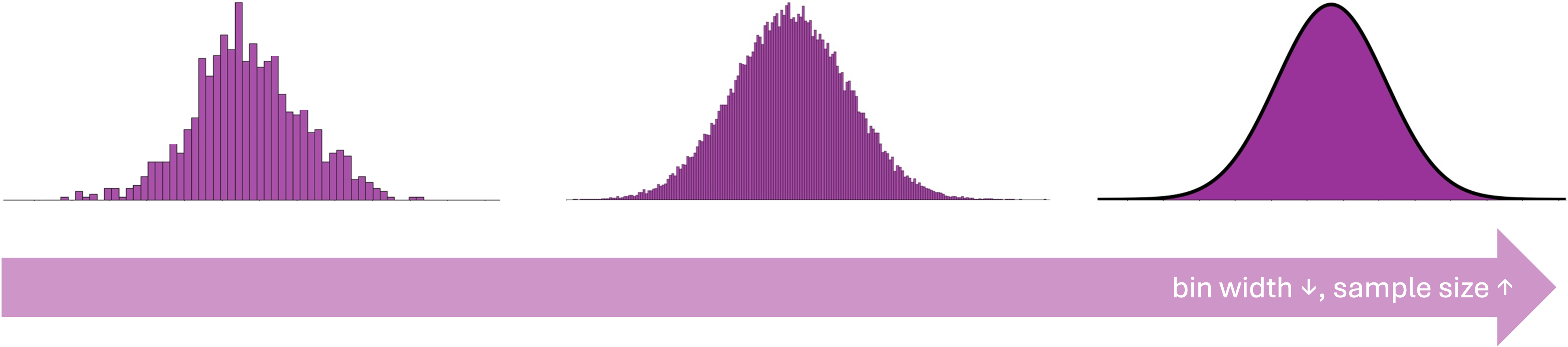
Fig. 6.1 Evolution from histogram to a probability density function
Mathematical Definition
A probability density function (PDF) for a continuous random variable \(X\), denoted \(f_X(x)\), specifies how “dense” the probability is around each point.
Mathematically,
Interpreting a PDF
It is important to note that \(f_X\) evaluated at any point \(x\) tells us about the relative likelihood of values in that neighborhood. Suppose a random variable \(X\) gives \(f_X(5.8) = 3\) and \(f_X(6.2) = 1\). We observe that:
Values in a small neighborhood around 5.8 are three times more likely to occur than values in the neighborhood of 6.2.
\(f_X\) does NOT give probabilities directly. \(f_X(6.2) = 1\) does NOT mean that the exact value of 6.2 occurs with probability 1.
Evaluations of \(f_X\) are not restricted to be at most 1. The set of rules for validity of a PDF will be discussed below.
Support
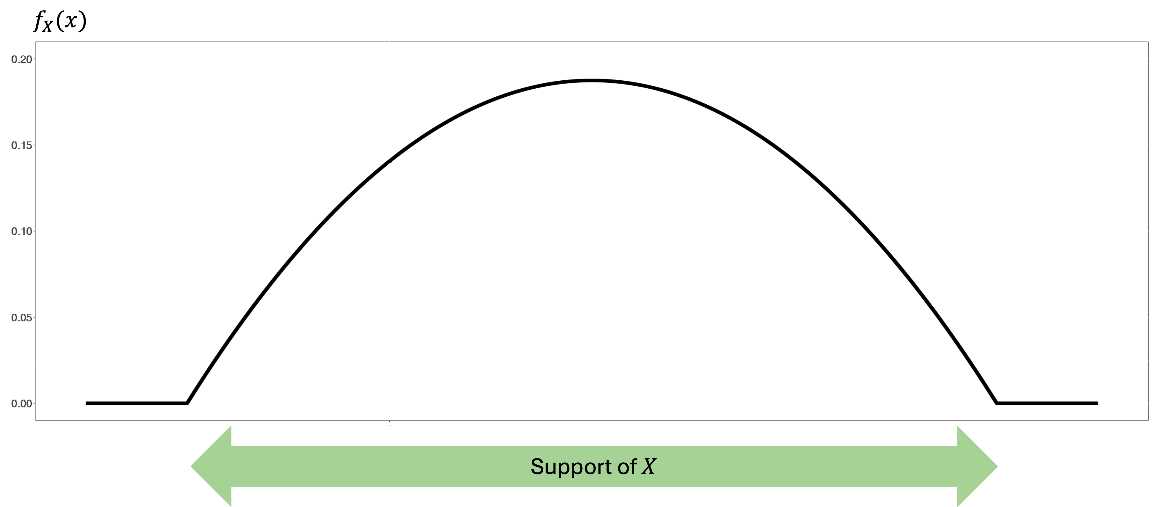
The support of a continuous random variable \(X\) is the set of all possible values that \(X\) can take, or equivalently, the set of values where its PDF is strictly positive:
6.1.3. Computing Probabilities: Areas Under the PDF
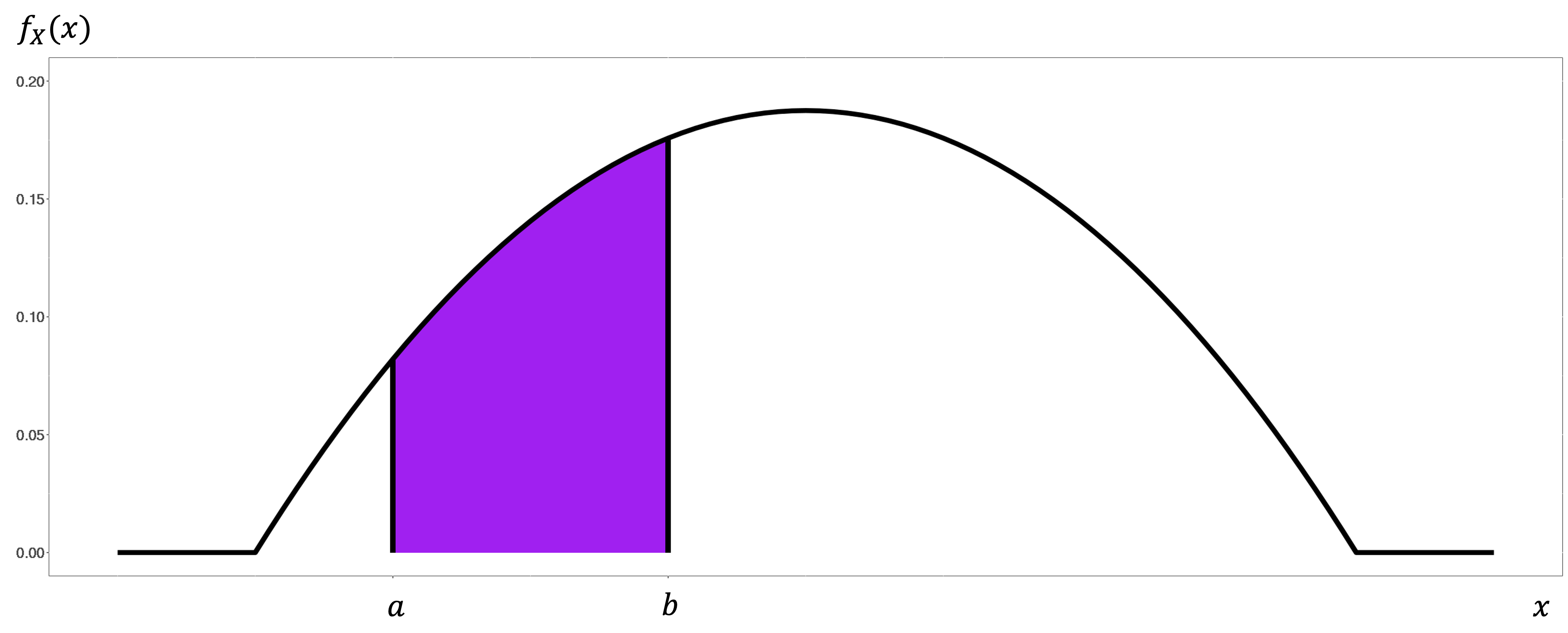
For a continuous random variable \(X\) with PDF \(f_X(x)\), the probability that \(X\) takes a value between \(a\) and \(b\) is equal to the area under \(f_X(x)\) between points \(a\) and \(b\). Mathematically,
Special Case: Probability at a Single Point
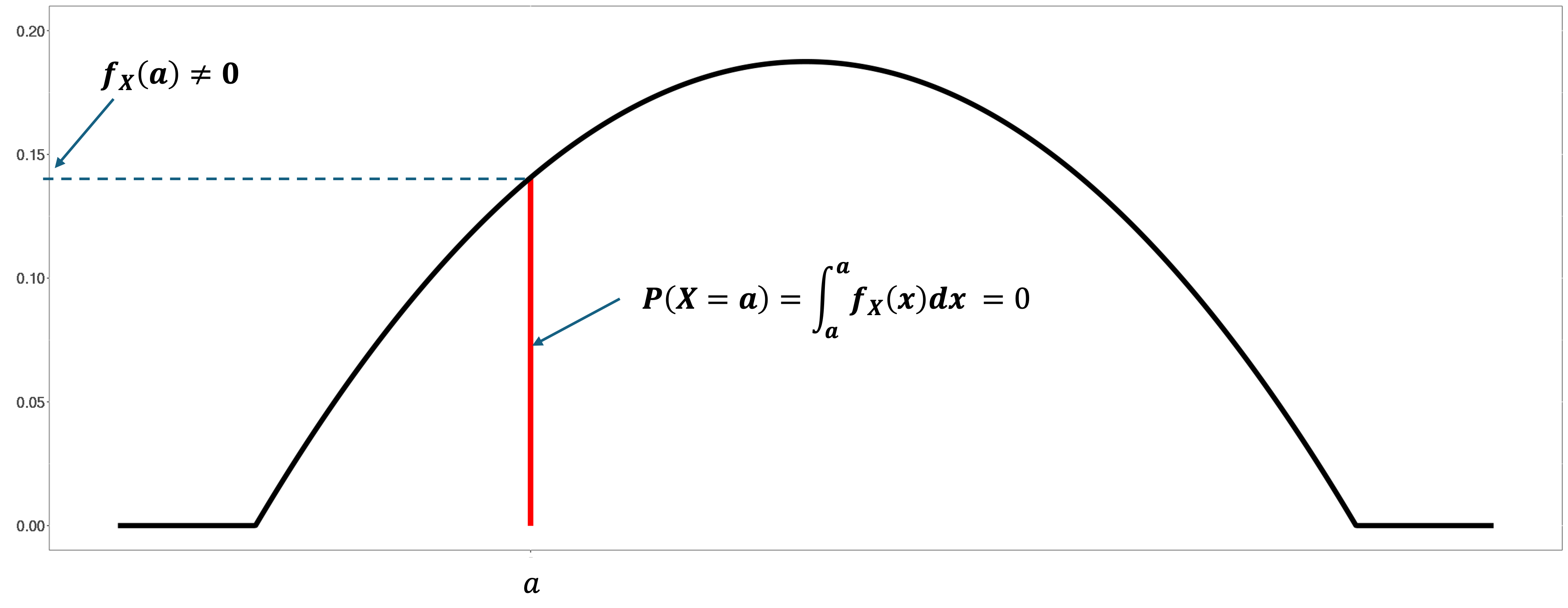
For any specific value \(a\),
Any integral from a point to itself is zero because the interval has zero width. Note that \(f_X(a)\) evaluated at any \(a\) in the support is positive. This again highlights the fact that evaluating \(f_X\) at a point does not directly give its probability.
An Important Consequence: Equality Doesn’t Matter
Since any single point has zero probability, using strict or weak inequalities does not affect the probabilities:
This is a major difference from discrete random variables, where \(P(X = k)\) could be positive, making the choice between \(<\) and \(\leq\) crucial.
6.1.4. Properties of A Valid Probability Density Function
Not every function can serve as a PDF. A valid PDF must satisfy two essential properties that parallel those required of discrete probability mass functions.
Property 1: Non-Negativity
A PDF must be non-negative everywhere. That is,
This makes sense—there cannot be a likelihood smaller than none. However, unlike discrete PMFs, PDFs are not constrained to values less than or equal to 1. They can take arbitrarily large values at some points, as long as they satisfy the next property.
Property 2: Total Area Equals One
The total area under a PDF must equal 1, or equivalently,
This implies that the probability of observing some value within the support is equal to 1.
Example💡: Validating and Working with a Simple PDF
Suppose the maximum diameter of a potato chip (\(X\)) produced at Factory A, in inches, follows the following probability density:
Identify the support of \(X\), sketch \(f_X(x)\), then verify that it is a legitimate PDF.
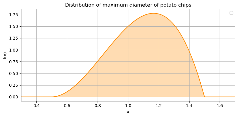
Fig. 6.2 Sketch of the PDF of maximum diameters of potato chips
\(\text{supp}(X) = [0.5, 1.5]\). \(f_X(x)\) takes a non-negative value at any \(x \in \mathbb{R}\) as evident from the sketch. We now verify that the integral of the PDF from \(-\infty\) to \(\infty\) equals 1:
\[\begin{split}\int_{-\infty}^\infty f_X(x)dx &= \int_{-\infty}^{0.5} f_X(x)dx + \int_{0.5}^{1.5}f_X(x)dx + \int_{1.5}^{\infty} f_X(x)dx\\ &= 0 + \int_{0.5}^{1.5} 12(x-0.5)^2(1.5-x) dx + 0\\\end{split}\]Above, we first split the beginning integral to a sum of integrals over three intervals. This step makes it evident that the integrals below \(0.5\) and above \(1.5\) are not just arbitrarily omitted from computation—they simply contribute zero area to the integral. Continuing,
\[\begin{split}&\int_{0.5}^{1.5} 12(x-0.5)^2(1.5-x) dx\\ &= \int_{0.5}^{1.5} (-12x^3 + 30x^2-21x + 4.5)dx\\ &=\frac{-12x^4}{4} + \frac{30x^3}{3} - \frac{21x^2}{2} + 4.5x \Bigg\rvert_{0.5}^{1.5}\\ &=-3x^4 + 10x^3 - 10.5x^2 + 4.5x \Bigg\rvert_{0.5}^{1.5}\\ &= 1.6875-0.6875 = 1.\end{split}\]Therefore, \(f_X\) satisfies both requirements for a valid PDF.
For a quality control procedure, managers of the factory has collected all the potato chips whose maximum diameter is smaller than 1”. What is the probability that a randomly selected potato chip in this pool has a maximum diameter greater than 0.8”?
The first task is to write the goal of the problem in correct probability statement. Since we have the information that the chips will always have a maximum diameter less than 1,
\[P(X > 0.8 | X < 1) = \frac{P(\{X > 0.8\} \cap \{X < 1 \})}{P(X < 1)}.\]The diameter can be greater than 0.8 and less than 1 only if it is between the two values. We simplify the numerator accordingly:
\[P(X > 0.8 | X < 1) = \frac{P(0.8 <X < 1)}{P(X < 1)}.\]Now integrate for each probability:
Numerator
\[\begin{split}P(0.8 < X < 1) &= \int_{0.8}^{1} f_X(x)dx \\ &=-3x^4 + 10x^3 - 10.5x^2 + 4.5x \Bigg\rvert_{0.8}^{1}\\ &=0.2288\end{split}\]Denominator
The denominator only has an upper boundary. This is equivalent to having a lower boundary of negative infinity, which gives us
\[\begin{split}P(X < 1) &= \int_{-\infty}^{1} f_X(x)dx = \int_{0.5}^1 f_X(x)dx\\\end{split}\]The final step above is true because the integral of \(f_X(x)\) in any region below \(0.5\) results in 0. Continuing,
\[P(X < 1) =-3x^4 + 10x^3 - 10.5x^2 + 4.5x \Bigg\rvert_{0.5}^{1} = 0.3125\]
Finally,
\[P(X > 0.8 | X < 1) = \frac{0.2288}{0.3125} = 0.73216\]
6.1.5. Important Types of Problems involving PDFs
A. Handling Complex Distributions
Real-world continuous distributions aren’t always described by simple functions. Common examples of more complex distributions are:
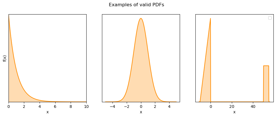
Fig. 6.3 A legitimate PDF can have many different functional forms
PDFs with one or both ends of the support extending to infinity (left two on Fig. 6.3)
PDFs of this type usually includes an exponential function. Make sure to review integration of simple exponential functions.
Piecewise-defined PDFs taking different functional forms over different regions of the support (right on Fig. 6.3)
When dealing with piecewise PDFs,
Identify all boundaries where the function forms change.
Break down any integrals spanning multiple regions into a sum of integrals, each spanning only a single region.
Example💡: A Piecewise-defined PDF
A professor of STAT 1234 drops by a coffee shop on campus before or after his 50-minute lecture. Suppose the time he enters the coffee shop has a PDF shown below. The time \(x\) is expressed in minutes relative to the start time of his lecture.
What is the probability that the professor enters the coffee shop within 3 minutes from his lecture?
We are looking for
This interval spans three regions:
part of the first non-trivial region where \(-3 \leq x\leq 0\),
the middle region \(0 \leq x\leq 50\) where the PDF is zero, then
part of the second non-trivial region where \(50\leq x\leq 53\).
We must break up the integral into three pieces accordingly:
B. Completing a Partially Known PDF
Sometimes we encounter functions that have the right shape to be PDFs but don’t integrate to 1. We must fix this by finding an appropriate normalization constant.
Example💡: Finding the Normalization Constant
Suppose we have a function:
Q: What is the constant \(k\) which makes \(kg(x)\) a valid PDF?
We need to find \(k\) such that \(\int_{-\infty}^{\infty} kg(x) \, dx = 1\).
First, we compute the integral of \(g(x)\).
\[\int_{-\infty}^{\infty}g(x)dx = \int_{0}^{2} x^2 \, dx = \left[\frac{x^3}{3}\right]_0^2 = \frac{8}{3}.\]To make the total area equal 1, we need
\[k \frac{8}{3} = 1 \implies k = \frac{3}{8}.\]Therefore, the valid PDF is:
\[\begin{split}f_X(x) = \begin{cases} \frac{3}{8}x^2 & \text{for } 0 \leq x \leq 2 \\ 0 & \text{elsewhere} \end{cases}.\end{split}\]
6.1.6. Bringing It All Together
The transition from discrete to continuous random variables represents a fundamental shift in thinking. Instead of asking “what’s the probability of exactly this value?” we ask “what’s the probability of values in this range?” This change enables us to model the rich variety of measurement data we encounter.
Key Takeaways 📝
Continuous random variables model measurable quantities that can take any value within an interval, unlike discrete variables that count distinct outcomes.
Probability density functions (PDFs) describe how probability is distributed across the continuous range, with higher values indicating more likely regions.
Probabilities are areas under the PDF, computed using integration: \(P(a < X < b) = \int_a^b f_X(x) \, dx\).
Individual points have probability zero for continuous variables—only intervals have positive probability.
Valid PDFs must be non-negative everywhere and integrate to 1 over their entire support.
In the next section, we’ll explore how to calculate expected values and variances for continuous random variables, extending the concepts we mastered in the discrete case.
6.1.7. Exercises
These exercises develop your skills in working with probability density functions, computing probabilities through integration, and verifying PDF validity.
Exercise 1: Validating and Computing Probabilities with a Basic PDF
A mechanical engineer models the deviation \(X\) (in millimeters) of a machined component from its target dimension. Based on production data, the PDF is:
Verify that \(f_X(x)\) is a valid PDF by checking both required properties.
Sketch the PDF. What shape does it have? Is it symmetric?
Find \(P(-0.5 \leq X \leq 0.5)\), the probability that the deviation is within half a millimeter of target.
Find \(P(X > 0)\). Does your answer make sense given the symmetry?
Find \(P(X = 0.3)\).
Solution
Part (a): Verify PDF validity
Property 1: Non-negativity
We need \(f_X(x) \geq 0\) for all \(x\). On the support \([-1, 1]\):
At \(x = 0\): \(f_X(0) = \frac{3}{4}(1-0) = \frac{3}{4} > 0\)
At \(x = \pm 1\): \(f_X(\pm 1) = \frac{3}{4}(1-1) = 0 \geq 0\)
For \(-1 < x < 1\): since \(|x| < 1\), we have \(x^2 < 1\), so \(1 - x^2 > 0\)
Therefore, \(f_X(x) \geq 0\) everywhere. ✓
Property 2: Total area equals 1
Both properties are satisfied, so \(f_X(x)\) is a valid PDF.
Part (b): Sketch and shape
The PDF is a downward-opening parabola with:
Maximum at \(x = 0\) where \(f_X(0) = \frac{3}{4}\)
Zeros at \(x = \pm 1\)
The function is symmetric about \(x = 0\) since \(f_X(-x) = \frac{3}{4}(1 - (-x)^2) = \frac{3}{4}(1 - x^2) = f_X(x)\).
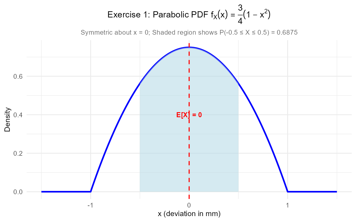
Part (c): P(-0.5 ≤ X ≤ 0.5)
About 68.75% of components have deviations within ±0.5 mm.
Part (d): P(X > 0)
By symmetry of \(f_X(x)\) about \(x = 0\):
This makes sense—the symmetric PDF assigns equal probability to positive and negative deviations.
Part (e): P(X = 0.3)
For any continuous random variable:
Any single point has probability zero for continuous random variables, even though \(x = 0.3\) is in the support and has positive density.
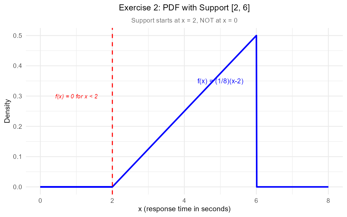
Exercise 2: PDF with Non-Zero Starting Point (Support Not Starting at 0)
A biomedical engineer studies the response time \(X\) (in seconds) of a nerve impulse. The PDF is:
Note that the support begins at \(x = 2\), not \(x = 0\).
Verify this is a valid PDF.
Find \(P(3 \leq X \leq 5)\) by direct integration.
Find \(P(X > 4)\).
Common Mistake Alert: A student incorrectly computes \(P(X \leq 4)\) by integrating \(\int_0^4 f_X(x) \, dx\). Explain their error and compute the correct value.
Solution
Part (a): Verify PDF validity
Non-negativity: On \([2, 6]\), since \(x \geq 2\), we have \(x - 2 \geq 0\), so \(f_X(x) = \frac{1}{8}(x-2) \geq 0\). ✓
Total area equals 1:
Part (b): P(3 ≤ X ≤ 5) by direct integration
Part (c): P(X > 4)
Part (d): Common Mistake Explanation
The student’s error: They integrated from 0, but the PDF equals 0 for \(x < 2\). The correct approach:
Key insight: When computing probabilities, only the region where \(f_X(x) > 0\) contributes. When the support doesn’t start at 0, be careful to integrate from the actual start of the support.
Exercise 3: Piecewise PDF with Multiple Regions
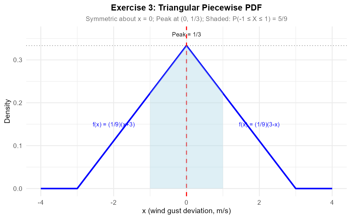
An aerospace engineer models wind gust intensity \(X\) (in m/s deviation from average) with the following PDF:
Verify this is a valid PDF. What is the geometric shape?
Use geometry (not calculus) to find \(P(-1 \leq X \leq 1)\).
Find \(P(X > 1)\) using integration.
Find the probability that the wind gust intensity exceeds 1 m/s given that it is positive: \(P(X > 1 | X > 0)\).
Solution
Part (a): Verify PDF and identify shape
The PDF forms a triangle with:
Vertex at \((0, \frac{3}{9}) = (0, \frac{1}{3})\)
Base from \(x = -3\) to \(x = 3\) (length = 6)
Non-negativity: Both pieces are non-negative on their respective domains. ✓
Total area = 1 (using triangle area formula):
Part (b): Geometric probability calculation
The region \(-1 \leq x \leq 1\) forms a trapezoid inside the triangle.
At \(x = -1\): \(f_X(-1) = \frac{1}{9}(-1+3) = \frac{2}{9}\)
At \(x = 0\): \(f_X(0) = \frac{1}{3}\)
At \(x = 1\): \(f_X(1) = \frac{1}{9}(3-1) = \frac{2}{9}\)
Alternative geometric approach:
Total triangle area = 1. The triangles outside \([-1, 1]\):
Left triangle (\(-3 \leq x \leq -1\)): base = 2, height = \(\frac{2}{9}\), area = \(\frac{1}{2} \times 2 \times \frac{2}{9} = \frac{2}{9}\)
Right triangle (\(1 \leq x \leq 3\)): base = 2, height = \(\frac{2}{9}\), area = \(\frac{2}{9}\)
Part (c): P(X > 1) using integration
Part (d): Conditional probability P(X > 1 | X > 0)
By symmetry: \(P(X > 0) = 0.5\)
From part (c): \(P(X > 1) = \frac{2}{9}\)
Exercise 4: Finding the Normalizing Constant
A chemical engineer proposes the following function to model reaction time \(X\) (in minutes):
where \(c\) is an unknown constant.
Find the value of \(c\) that makes \(g(x)\) a valid PDF.
With this value of \(c\), find \(P(1 \leq X \leq 3)\).
Sketch the PDF. Where is the mode (peak) of this distribution?
Solution
Part (a): Find normalizing constant c
For a valid PDF, \(\int_{-\infty}^{\infty} g(x) \, dx = 1\):
Part (b): P(1 ≤ X ≤ 3)
Part (c): Sketch and mode
The function \(f_X(x) = \frac{3}{32}(4x - x^2) = \frac{3}{32}x(4-x)\) is a downward-opening parabola.
To find the mode, take the derivative and set to zero:
Solving: \(x = 2\)
The mode is at x = 2 minutes, where \(f_X(2) = \frac{3}{32}(8 - 4) = \frac{3}{8}\).
Exercise 5: Piecewise PDF with Gap in Support
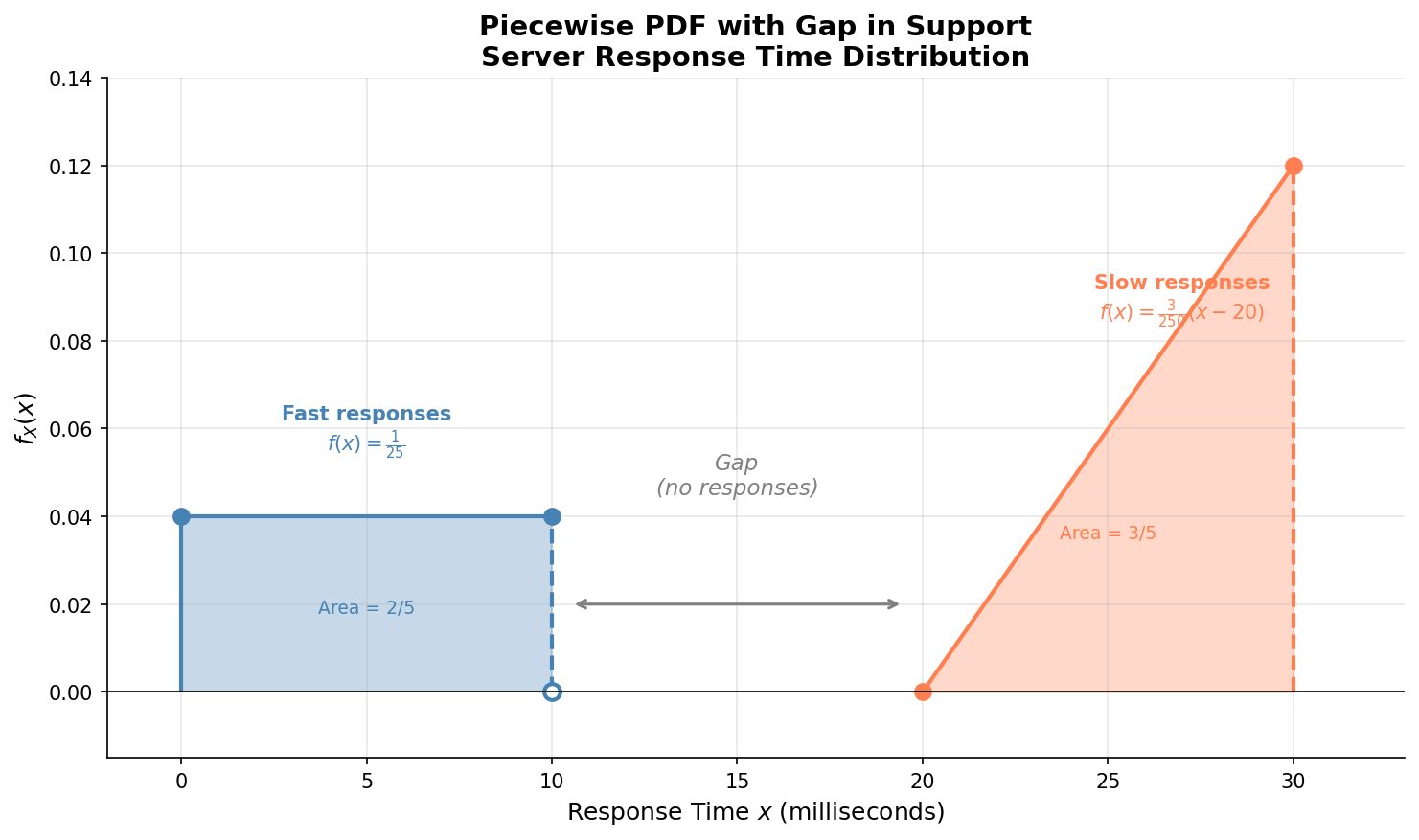
A data scientist models server response categories with the following PDF for response time \(X\) (in milliseconds):
Note the gap in support from \(x = 10\) to \(x = 20\) (no responses in this range).
Verify this is a valid PDF.
Find \(P(5 < X < 25)\). Be careful with the gap!
What percentage of responses are “fast” (under 10 ms)?
Given that a response is in the “slow” category (\(X \geq 20\)), what is \(P(X > 25 | X \geq 20)\)?
Solution
Part (a): Verify PDF validity
Non-negativity:
Region 1: \(\frac{1}{25} > 0\) ✓
Region 2: For \(20 \leq x \leq 30\), \(x - 20 \geq 0\), so \(\frac{3}{250}(x-20) \geq 0\) ✓
Total area = 1:
Total: \(\frac{2}{5} + \frac{3}{5} = 1\) ✓
Part (b): P(5 < X < 25)
This spans multiple regions. We need:
Calculate each part:
Part (c): Percentage of fast responses
Part (d): Conditional probability P(X > 25 | X ≥ 20)
Since slow responses are in the region \([20, 30]\):
Exercise 6: Exponential-Type Function
A reliability engineer models component lifetime \(X\) (in years) with PDF:
Find the constant \(c\) that makes this a valid PDF.
Find \(P(X > 3)\), the probability a component lasts more than 3 years.
Find \(P(1 < X < 4)\).
If a component has already lasted 2 years, what is \(P(X > 5 | X > 2)\)?
Solution
Part (a): Find c
Therefore, \(c = \frac{1}{2}\).
The PDF is \(f_X(x) = \frac{1}{2}e^{-x/2}\) for \(x \geq 0\).

Part (b): P(X > 3)
Part (c): P(1 < X < 4)
Part (d): Conditional probability (Memoryless property)
This is an exponential distribution with rate \(\lambda = \frac{1}{2}\). By the memoryless property:
The probability of surviving an additional 3 years is the same regardless of how long the component has already lasted—this is the defining characteristic of exponential distributions.
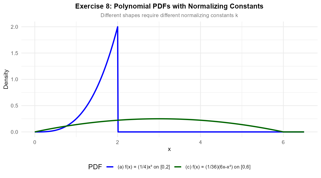
Exercise 7: Finding Normalizing Constants — Polynomial Functions
For each of the following functions, find the constant \(k\) that makes it a valid PDF.
\(g(x) = kx^3\) for \(0 \leq x \leq 2\), and 0 elsewhere.
\(g(x) = k(x - 1)^2\) for \(1 \leq x \leq 4\), and 0 elsewhere.
\(g(x) = k(6x - x^2)\) for \(0 \leq x \leq 6\), and 0 elsewhere.
\(g(x) = k\sqrt{x}\) for \(0 \leq x \leq 9\), and 0 elsewhere.
Solution
Part (a): g(x) = kx³ on [0, 2]
For a valid PDF: \(\int_{0}^{2} kx^3 \, dx = 1\)
Therefore, \(k = \frac{1}{4}\).
Verification: \(f_X(x) = \frac{1}{4}x^3 \geq 0\) on \([0, 2]\). ✓
Part (b): g(x) = k(x-1)² on [1, 4]
Therefore, \(k = \frac{1}{9}\).
Part (c): g(x) = k(6x - x²) on [0, 6]
Therefore, \(k = \frac{1}{36}\).
Verification of non-negativity: \(6x - x^2 = x(6-x) \geq 0\) for \(0 \leq x \leq 6\). ✓
Part (d): g(x) = k√x on [0, 9]
Therefore, \(k = \frac{1}{18}\).
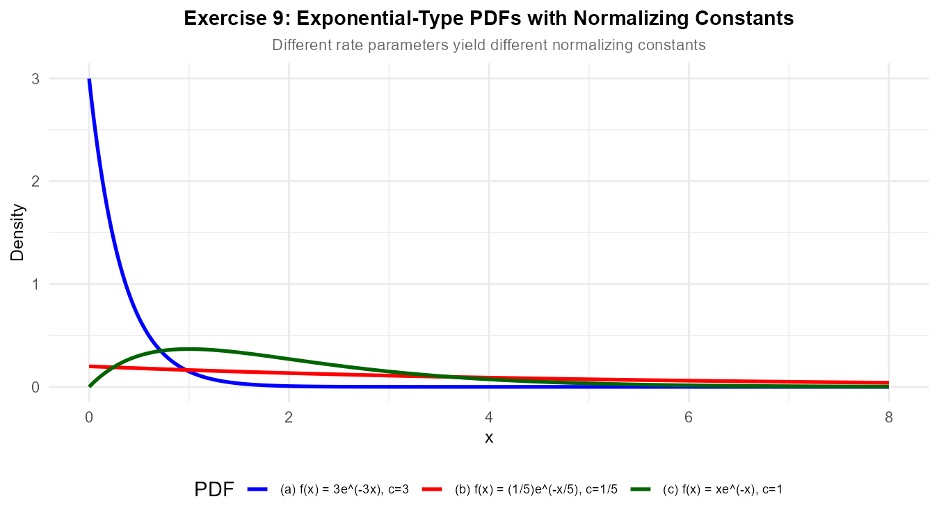
Exercise 8: Finding Normalizing Constants — Exponential Functions
For each of the following functions, find the constant \(c\) that makes it a valid PDF.
\(g(x) = ce^{-3x}\) for \(x \geq 0\), and 0 elsewhere.
\(g(x) = ce^{-x/5}\) for \(x \geq 0\), and 0 elsewhere.
\(g(x) = cxe^{-x}\) for \(x \geq 0\), and 0 elsewhere. (Hint: Use integration by parts)
\(g(x) = ce^{-(x-2)}\) for \(x \geq 2\), and 0 elsewhere. (Note: Support starts at 2, not 0)
Solution
Part (a): g(x) = ce^{-3x} for x ≥ 0
Therefore, \(c = 3\).
The PDF is \(f_X(x) = 3e^{-3x}\) for \(x \geq 0\) (Exponential with rate \(\lambda = 3\)).
Part (b): g(x) = ce^{-x/5} for x ≥ 0
Therefore, \(c = \frac{1}{5}\).
The PDF is \(f_X(x) = \frac{1}{5}e^{-x/5}\) for \(x \geq 0\) (Exponential with rate \(\lambda = \frac{1}{5}\), or mean \(\mu = 5\)).
Part (c): g(x) = cxe^{-x} for x ≥ 0
Use integration by parts with \(u = x\), \(dv = e^{-x}dx\):
Then \(du = dx\), \(v = -e^{-x}\).
Therefore, \(c = 1\).
The PDF is \(f_X(x) = xe^{-x}\) for \(x \geq 0\). This is a Gamma distribution with shape \(\alpha = 2\) and rate \(\beta = 1\).
Part (d): g(x) = ce^{-(x-2)} for x ≥ 2
The support starts at \(x = 2\), so we integrate from 2:
Therefore, \(c = 1\).
The PDF is \(f_X(x) = e^{-(x-2)}\) for \(x \geq 2\). This is a shifted exponential distribution.
Exercise 9: Piecewise Triangular PDF
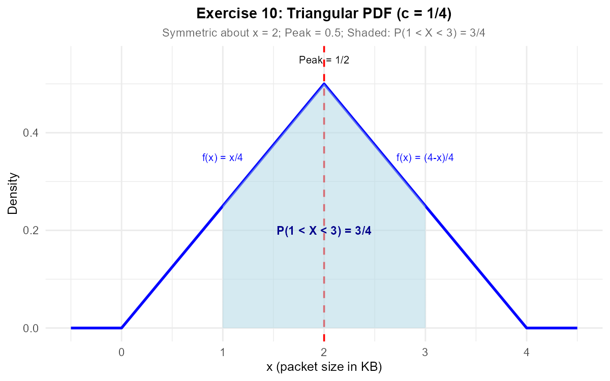
A computer scientist models network packet sizes \(X\) (in kilobytes) with the following proposed density:
Find the constant \(c\) that makes this a valid PDF.
Sketch the PDF. What shape is it?
Find \(P(1 < X < 3)\).
Find \(P(X > 3)\).
Solution
Part (a): Find normalizing constant c
The PDF must integrate to 1 over the entire support:
First integral:
Second integral:
Total: \(2c + 2c = 4c = 1\), so \(c = \frac{1}{4}\).
Part (b): Sketch and shape
The PDF forms a triangle with:
Base from \(x = 0\) to \(x = 4\) (length = 4)
Peak at \(x = 2\) where \(f_X(2) = \frac{1}{4} \cdot 2 = \frac{1}{2}\)
Verification using triangle area: \(\frac{1}{2} \times 4 \times \frac{1}{2} = 1\) ✓
Part (c): P(1 < X < 3)
This spans both pieces of the PDF:
Part (d): P(X > 3)
6.1.8. Additional Practice Problems
True/False Questions (1 point each)
For a continuous random variable, \(P(X = a) = f_X(a)\) where \(f_X\) is the PDF.
Ⓣ or Ⓕ
If \(f_X(x) = 0.5\) for \(2 \leq x \leq 4\) and 0 elsewhere, then this is a valid PDF.
Ⓣ or Ⓕ
For continuous random variables, \(P(a < X < b) = P(a \leq X \leq b)\).
Ⓣ or Ⓕ
For a valid PDF, \(f_X(x) \leq 1\) for all \(x\).
Ⓣ or Ⓕ
If \(g(x) = kx^2\) for \(0 \leq x \leq 3\) is a valid PDF, then \(k = \frac{1}{9}\).
Ⓣ or Ⓕ
If \(g(x) = ce^{-2x}\) for \(x \geq 0\) is a valid PDF, then \(c = 2\).
Ⓣ or Ⓕ
Multiple Choice Questions (2 points each)
For \(f_X(x) = 3x^2\) on \([0, 1]\), what is \(P(X > 0.5)\)?
Ⓐ 0.125
Ⓑ 0.5
Ⓒ 0.75
Ⓓ 0.875
For a continuous random variable with PDF symmetric about \(x = 5\) on support \([0, 10]\), what is \(P(X < 5)\)?
Ⓐ 0.25
Ⓑ 0.5
Ⓒ 0.75
Ⓓ Cannot determine without the specific PDF
What value of \(k\) makes \(g(x) = k(4 - x^2)\) a valid PDF on \([-2, 2]\)?
Ⓐ \(k = \frac{1}{32}\)
Ⓑ \(k = \frac{3}{32}\)
Ⓒ \(k = \frac{1}{16}\)
Ⓓ \(k = \frac{3}{16}\)
What value of \(c\) makes \(g(x) = ce^{-x/4}\) a valid PDF on \([0, \infty)\)?
Ⓐ \(c = 4\)
Ⓑ \(c = \frac{1}{4}\)
Ⓒ \(c = e^{-4}\)
Ⓓ \(c = 1\)
If \(g(x) = k(x-1)(5-x)\) for \(1 \leq x \leq 5\) is a valid PDF, what is \(k\)?
Ⓐ \(k = \frac{1}{32}\)
Ⓑ \(k = \frac{3}{32}\)
Ⓒ \(k = \frac{1}{16}\)
Ⓓ \(k = \frac{3}{16}\)
For \(f_X(x) = \frac{3}{8}x^2\) on \([0, 2]\), what is \(P(X < 1)\)?
Ⓐ \(\frac{1}{8}\)
Ⓑ \(\frac{1}{4}\)
Ⓒ \(\frac{3}{8}\)
Ⓓ \(\frac{1}{2}\)
Answers to Practice Problems
True/False Answers:
False — \(f_X(a)\) is the density at point \(a\), NOT the probability. \(P(X = a) = 0\) for continuous random variables.
True — The function is non-negative, and \(\int_2^4 0.5 \, dx = 0.5 \times 2 = 1\). ✓
True — For continuous random variables, individual points have probability zero, so including or excluding the endpoints doesn’t change the probability.
False — PDFs can exceed 1 as long as the total area equals 1. For example, \(f_X(x) = 4\) for \(0 \leq x \leq 0.25\) is valid.
True — \(\int_0^3 kx^2 \, dx = k[\frac{x^3}{3}]_0^3 = k \cdot 9 = 1\), so \(k = \frac{1}{9}\). ✓
True — \(\int_0^\infty ce^{-2x} \, dx = c \cdot [-\frac{1}{2}e^{-2x}]_0^\infty = c \cdot \frac{1}{2} = 1\), so \(c = 2\). ✓
Multiple Choice Answers:
Ⓓ — \(P(X > 0.5) = \int_{0.5}^{1} 3x^2 \, dx = [x^3]_{0.5}^{1} = 1 - 0.125 = 0.875\).
Ⓑ — By symmetry about \(x = 5\), exactly half the probability is below 5 and half above. \(P(X < 5) = 0.5\).
Ⓑ — \(\int_{-2}^{2} k(4 - x^2) \, dx = k[4x - \frac{x^3}{3}]_{-2}^{2} = k[(8 - \frac{8}{3}) - (-8 + \frac{8}{3})] = k \cdot \frac{32}{3} = 1\), so \(k = \frac{3}{32}\).
Ⓑ — \(\int_0^\infty ce^{-x/4} \, dx = c[-4e^{-x/4}]_0^\infty = c \cdot 4 = 1\), so \(c = \frac{1}{4}\).
Ⓑ — First expand: \((x-1)(5-x) = -x^2 + 6x - 5\). Integrate:
\(\int_1^5 k(-x^2 + 6x - 5) \, dx = k[-\frac{x^3}{3} + 3x^2 - 5x]_1^5\)
\(= k[(-\frac{125}{3} + 75 - 25) - (-\frac{1}{3} + 3 - 5)] = k[(-\frac{125}{3} + 50) - (-\frac{7}{3})]\)
\(= k[\frac{-125 + 150 + 7}{3}] = k \cdot \frac{32}{3} = 1\)
So \(k = \frac{3}{32}\).
Ⓐ — \(P(X < 1) = \int_0^1 \frac{3}{8}x^2 \, dx = \frac{3}{8} \cdot \frac{x^3}{3}\Big|_0^1 = \frac{1}{8}\).