Slides 📊

2.1. Data Set Structure and Variable Types

Imagine being handed a spreadsheet containing thousands of numbers—sales figures, temperature readings, or survey responses. Without organization and visualization, these numbers remain just that: a collection of digits offering little immediate insight.

A raw data file is essentially a laundry list of values. This chapter introduces you to the basic vocabulary of structured data sets and demonstrates how tables, pie charts, bar graphs, and histograms transform data values into intuitve patterns. We begin by establishing a common language for organizing and describing a data set.

Road Map 🧭

Define case and variable, and understand how they are organized in a rectangular data set.
Define categorical (qualitative) and numerical (quantitative) variables and learn their further divisions.
Understand that each variable type requires a different set of summarizing tools to reflect its unique structure.

2.1.1. Understanding the Structure of a Data Set

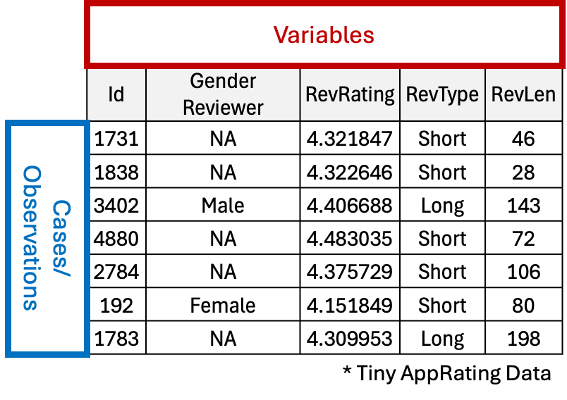
cases and variables in a rectangular spreadsheet — Fig. 2.1 Cases and variables in a rectangular spreadsheet

Before delving into visualization techniques, we need to understand how data is organized. A data set is typically arranged as a rectangular array where

rows represent cases or observations (individual entities such as people, cities, or products), and
columns represent variables (specific attributes of each case).

When examining any data set, always begin by asking the three fundamental questions:

Who? - What cases does the data describe? How many cases are there?
What? - Which variables are being measured, with what units, and on what scale? How many variables are there?
Why? - What question motivated the data, and are the variables appropriate for answering that question?

These questions may seem simple, but they provide essential context for any statistical analysis. Without understanding their answers, we risk misinterpreting results or drawing inappropriate conclusions.

2.1.2. Variable Classification

Variables come in different types, each with its own properties and appropriate summarizing methods. Fig. 2.2 illustrates the primary classification system:

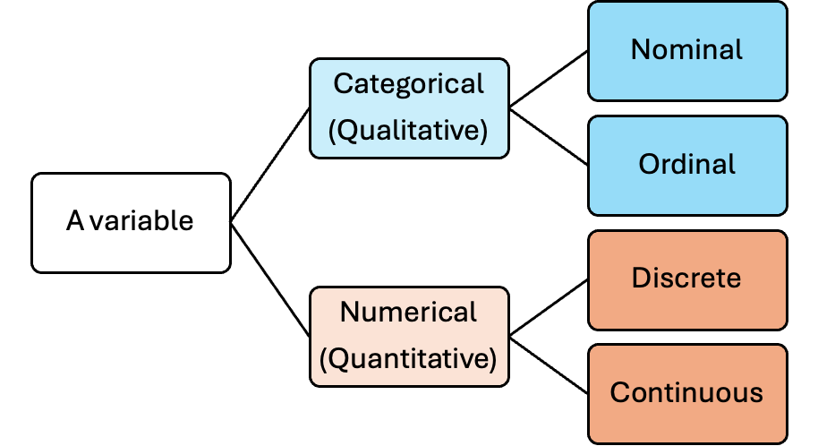
Flow-chart of variable types — Fig. 2.2 Variable types flow chart

Categorical (Qualitative) Variables

A categorical variable describes an attribute which can be classified into distinct categories. Typically, these categories are distinguished by names or labels and cannot be measured on a numerical scale. It can be further divided into:

Nominal variables: categories with no inherent order (e.g., fruit types, car brands, hair colors)

Ordinal variables: categories with a meaningful order but uneven or unmeasurable spacing between values (e.g., education levels, survey responses on a scale from “strongly disagree” to “strongly agree”)

Numerical (Quantitative) Variables

A numerical variable records measurements or counts that can be expressed on a numerical scale. It can be subdivided into:

Discrete variables: variables whose possible outcomes are separate, distinct points with no possible values between consecutive units (e.g., number of books on a shelf, number of students in a classroom)

Continuous variables: variables that can take any value within a range, limited only by measurement precision (e.g., height, weight, temperature, time)

A Tip 🔎: When confused bewteen discrete and continuous…🤔

Take any single value from the numerical variable. Then ask, can I clearly identify the “next” (or “previous”) point?

If yes, then discrete

If no, then continuous

For example:

If there are three students in a classroom now, what is the “next” possible value for the student count? Without question, it’s four. → discrete

If the current temperature is 81 degrees Fahrenheit, what is the “next” value it can be? 82? 81.1? 81.00001? Not clear. → continuous

A quantitavie variable can also be classifed as measured on an interval scale or a ratio scale:

Comparison of quantitative variables on interval vs ratio scale
Property	Interval scale	Ratio scale
True zero	Has no true zero point. Its “zero” value does not imply the absence of the quanity being measured	Has meaningful zero that represents the absence of the quantity
Ratios	Ratios of values do not have a meaning.	Ratios of values make sense.
Examples	Celsius temperature: 0 degrees Celcius does not imply any absence. SAT score: If two students received 800 and 1600 on SAT, it does not mean that the second student did twice as well.	height, weight, time, etc. If two animal species have average heights of 1 foot and 2 feet, respectively, then it means that the second species is twice as tall as the first, on average.

Example 💡: Variable Type Depends on Both Nature and Context

When classifying a variable, its definition given by the data collector is just as important as its naturally occurring properties. Take the final exam grades of an imaginary course, MATH 1234, for example.

Researcher 1 records the data as percentage scores after a curve has been applied (Variable 1).
Researcher 2 records the data as belonging to one of the intervals 0%-60%, 60%-70%, 70%-80%, then 80%-100% (Variable 2).

Although both variables come from the same source, they are now of distinct types:

Variable 1 is a continuous numerical variable on an interval scale. A grade of 0% has lost its meaning due to the curve. Also, a student with 80% did not perform twice as better as one with 40%.
Variable 2 is an ordinal categorical variable. Although a natural order exists among the intervals, no meaningful arithmetic oprations are possible between them, indicating that they are not numerical values.

In general cases where no experimental details are given, you may focus on the variable’s natural properties. However, when additional context is available, it must be factored into how you classify it.

2.1.3. Bringing It All Together

Key Takeaways 📝

Always identify the who, what and why in a dataset.
Be able to classify a variable by considering both its natural properties and its specific usage in an experiment.

2.1.4. Exercises

These exercises build your understanding of data organization and variable classification—foundational skills for all statistical analysis. Each exercise connects to real-world scenarios relevant to engineering, computer science, and applied sciences.

A Note on These Exercises

These exercises are designed to build your understanding progressively:

Exercise 1 practices the fundamental questions (Who? What? Why?) that frame every data analysis
Exercise 2 develops skill in distinguishing categorical from numerical variables
Exercise 3 refines classification into nominal/ordinal and discrete/continuous
Exercise 4 explores the interval vs. ratio scale distinction for numerical variables
Exercise 5 demonstrates how context changes classification—the same measurement can be different variable types
Exercise 6 applies all concepts to a comprehensive real-world data set

Work through the hints before checking solutions—the reasoning process builds lasting understanding!

Exercise 1: The Three Fundamental Questions

Before analyzing any data set, statisticians ask three fundamental questions: Who? (What are the cases?), What? (What variables are measured?), and Why? (What question motivated the data collection?). This exercise practices identifying these elements.

Background: Cases and Variables

A data set is typically organized as a rectangular array where:

Rows represent cases (also called observations)—the individual entities being studied
Columns represent variables—the specific attributes measured for each case

Clearly identifying cases is crucial because it determines the unit of analysis and affects which statistical methods are appropriate.

Scenario A — Software Performance Testing

A quality assurance team at a software company records data on 150 automated test runs. For each test run, they record: the test ID, the module being tested (Authentication, Database, UI, or API), execution time in milliseconds, memory usage in MB, pass/fail status, and the build version number.

Who? Identify the cases in this data set. How many cases are there?
What? List all variables being measured. For each, identify the units (if applicable).
Why? What research questions might have motivated collecting this data?

Scenario B — Manufacturing Quality Control

An aerospace components manufacturer inspects turbine blades. Each blade is assigned a serial number, measured for length (mm), weight (grams), inspected for surface defects (None, Minor, Major), tested for tensile strength (MPa), and assigned a quality grade (A, B, C, or Reject).

Who? Identify the cases. What uniquely identifies each case?
What? List all variables. Which might be considered an identifier rather than a true variable?
Why? Propose two different research questions that could be addressed with this data.

Scenario C — Network Security Analysis

A cybersecurity team monitors network traffic, recording data on 10,000 connection attempts. For each attempt, they log: timestamp, source IP address, destination port number, packet size (bytes), protocol type (TCP, UDP, ICMP), and whether the connection was flagged as suspicious (Yes/No).

Who? What constitutes a single case in this study?
What? Identify all variables. Which variable might serve as a response variable in a classification model?
Why? How might the research question differ between a real-time intrusion detection system and a post-incident forensic analysis?

Solution

Part (a): Software Testing — Cases

The cases are the individual test runs. There are 150 cases in the data set.

Note: The cases are NOT the modules, even though modules are recorded. Each row represents one test run, and the same module can appear in multiple rows.

Part (b): Software Testing — Variables

Variable	Description	Units
Test ID	Unique identifier for each test	(identifier, no units)
Module	Component being tested	(categories: Auth, DB, UI, API)
Execution time	How long the test took	milliseconds (ms)
Memory usage	RAM consumed during test	megabytes (MB)
Pass/fail status	Test outcome	(categories: Pass, Fail)
Build version	Software version tested	(version number)

Part (c): Software Testing — Research Questions

Possible research questions include:

Do certain modules consistently take longer to test or use more memory?
Is there a relationship between execution time and memory usage?
Do newer build versions have higher pass rates?
Which modules have the highest failure rates?

Part (d): Manufacturing — Cases

The cases are the individual turbine blades. Each blade is uniquely identified by its serial number.

Part (e): Manufacturing — Variables

Variable	Notes
Serial number	Identifier (not a true variable for analysis)
Length	Measurement variable (mm)
Weight	Measurement variable (grams)
Surface defects	Categorical variable (None/Minor/Major)
Tensile strength	Measurement variable (MPa)
Quality grade	Categorical variable (A/B/C/Reject)

The serial number is an identifier, not a variable of interest. It uniquely labels each case but carries no analytical meaning—we wouldn’t compute an “average serial number.”

Part (f): Manufacturing — Research Questions

Predictive question: Can we predict quality grade from the physical measurements (length, weight, tensile strength)?
Quality control question: What proportion of blades have surface defects, and is there a relationship between defect severity and tensile strength?

Part (g): Network Security — Cases

The cases are the individual connection attempts. Each of the 10,000 connection attempts represents one case.

Part (h): Network Security — Variables

The variables are: timestamp, source IP, destination port, packet size, protocol type, and suspicious flag.

The suspicious flag (Yes/No) would likely serve as the response variable in a classification model, with the other variables serving as predictors.

Part (i): Network Security — Research Questions

Real-time detection: The question is predictive—“Given the characteristics of an incoming connection, should we flag it as suspicious?” Speed and false-positive rates are critical.
Forensic analysis: The question is descriptive/explanatory—“What patterns characterize the suspicious connections? Which IP addresses or ports were most commonly involved?” Thoroughness matters more than speed.

Exercise 2: Categorical vs. Numerical Classification

The first major distinction in variable classification is between categorical (qualitative) and numerical (quantitative) variables. This exercise develops your ability to make this fundamental distinction, including tricky cases where numbers don’t necessarily mean numerical.

Key Principle

Numbers don’t automatically make a variable numerical. A variable is numerical only if arithmetic operations (addition, subtraction, averaging) produce meaningful results. ZIP codes, jersey numbers, and ID numbers contain digits but are categorical—averaging them makes no sense.

For each variable below, classify it as categorical or numerical. Provide a brief justification focusing on whether arithmetic operations are meaningful.

The response time (in milliseconds) of a web server handling API requests.
The HTTP status code returned by a server (200, 404, 500, etc.).
The processor architecture of computers in a data center (x86, ARM, RISC-V).
The number of CPU cores in a server.
The MAC address of a network interface card.
The star rating (1-5 stars) given in app store reviews.
The temperature of a CPU under load, measured in degrees Celsius.
The version number of a software release (e.g., 2.4.1).
The employee ID number at a tech company.
The bandwidth of a network connection in Mbps.
The priority level of support tickets (Low, Medium, High, Critical).
The number of bugs found in a code review.

Solution

Part	Classification	Justification
	Numerical	Response time is a measurement of duration. Averaging response times (e.g., “mean response time was 45 ms”) is meaningful. Even if recorded as whole milliseconds, time is fundamentally continuous.
	Categorical	HTTP status codes are labels for categories of responses. The “average” of 200 and 404 (= 302) has no meaning. Code 302 exists but isn’t the “average” of success and not-found.
	Categorical	Architecture names are labels with no numerical interpretation.
	Numerical	This is a count of physical components. “One server has twice as many cores as another” is a meaningful statement.
	Categorical	MAC addresses are identifiers. Despite being hexadecimal numbers, arithmetic operations are meaningless.
	Categorical (ordinal)	While stars use numbers 1-5, the intervals between ratings may not be equal. Is the difference between 1 and 2 stars the same as between 4 and 5 stars? Typically treated as ordinal categorical. (Note: Some analysts treat such ratings as numerical for convenience, but strictly speaking, they are ordinal.)
	Numerical	Temperature is a physical measurement. Differences are meaningful (“10°C warmer”). Even if displayed as whole degrees, temperature could theoretically be 72.347°C.
	Categorical	Version numbers are labels. Version 2.0 is not “twice” version 1.0, and 2.4.1 cannot be meaningfully averaged with 3.1.0.
	Categorical	Employee IDs are identifiers, not quantities. The “average employee ID” is meaningless.
	Numerical	Bandwidth is a measurement of data transfer rate. “100 Mbps is twice as fast as 50 Mbps” is meaningful. As a rate, it’s fundamentally continuous.
	Categorical	Priority levels are ordered categories (labels), not measurements.
	Numerical	This is a count of discrete events. “We found twice as many bugs this sprint” is meaningful.

Key Insight: The presence of numbers does not make a variable numerical. Ask yourself: “Does it make sense to compute an average of these values?” If the answer is no, the variable is categorical.

Preview of Discrete vs. Continuous: Notice that some numerical variables above are counts (cores, bugs) while others are measurements (response time, temperature, bandwidth). This distinction becomes important in Exercise 3: counts are discrete, measurements are continuous.

Exercise 3: Sub-classification — Nominal/Ordinal and Discrete/Continuous

Once you’ve identified whether a variable is categorical or numerical, the next step is sub-classification:

Categorical variables are either nominal (no natural ordering) or ordinal (meaningful order exists)
Numerical variables are either discrete (countable, distinct values) or continuous (any value in a range)

The “Next Value” Test for Discrete vs. Continuous

For numerical variables, ask: “Can I clearly identify the next possible value?”

If yes → discrete (e.g., number of students: 3 → next is 4)
If no → continuous (e.g., temperature: 81°F → next could be 81.1, 81.01, 81.001…)

Apply this test to the theoretical scale, not the recorded precision:

After 81.0 bpm, what is the “next possible” heart rate? Is it 82? No—81.01 bpm is possible. Is it 81.01? No—81.001 is possible. The next value is not well-defined because infinitely many values exist between any two points → continuous
After 3 defects, what is the “next possible” count? It’s 4. There is no value between 3 and 4 defects → discrete

Classify by Potential, Not Recording Precision

Important: We classify variables based on what they could theoretically be, not how they happen to be recorded.

Heart rate is continuous because it’s a rate that could take any positive value (72.3 bpm), even though monitors often display integers
Time is continuous even if your stopwatch only shows whole seconds
Weight is continuous even if the scale rounds to the nearest pound

Ask: “If I had a perfect measuring instrument with unlimited precision, could this take non-integer values?” If yes → continuous.

For each variable, provide the complete classification: (Categorical Nominal, Categorical Ordinal, Numerical Discrete, or Numerical Continuous).

Part A: Software Engineering Context

The programming language used in a project (Python, Java, C++, Rust).
The number of commits to a repository in a day.
The code complexity rating (Low, Medium, High).
The execution time of a sorting algorithm in nanoseconds.
The number of dependencies in a software package.
The severity level of a security vulnerability (Informational, Low, Medium, High, Critical).

Part B: Mechanical Engineering Context

The material type of a component (Steel, Aluminum, Titanium, Carbon Fiber).
The number of fatigue cycles a part withstands before failure.
The surface roughness measurement (Ra) in micrometers.
The tolerance class of a bearing (P0, P6, P5, P4, P2 — in order of increasing precision).
The weight of a manufactured part in grams.
The number of defects found in a batch of 100 parts.

Part C: Biomedical Engineering Context

The blood type of a patient (A, B, AB, O).
The pain level reported by a patient (0-10 scale).
The heart rate in beats per minute.
The number of doses of medication administered.
The concentration of a drug in the bloodstream (mg/L).
The stage of a disease (Stage I, II, III, IV).

Solution

Part A: Software Engineering

Part	Classification	Reasoning
	Categorical Nominal	Programming languages are categories with no inherent order. Python isn’t “greater than” Java.
	Numerical Discrete	Commits are counted in whole numbers. After 5 commits, what’s the next possible value? Exactly 6—you cannot have 5.5 commits. The “next value” is well-defined → discrete. This is a count, which is inherently discrete.
	Categorical Ordinal	There’s a meaningful order (Low < Medium < High) but intervals aren’t quantifiable.
	Numerical Continuous	Time is a rate/duration that can theoretically take any positive value. After 150.5 ns, what’s the next possible value? 150.6? No—150.51 is possible. 150.51? No—150.501 is possible. The “next value” is undefined → continuous. Even if your timer only displays integers, execution time is fundamentally continuous.
	Numerical Discrete	Dependencies are counted. You can’t have 3.5 dependencies—this is inherently a whole number.
	Categorical Ordinal	Clear ordering exists (Informational < Low < … < Critical) but the “distance” between levels isn’t quantified.

Part B: Mechanical Engineering

Part	Classification	Reasoning
	Categorical Nominal	Material types are categories with no inherent order.
	Numerical Discrete	Fatigue cycles are counted in whole numbers. After 10,000 cycles, what’s the next possible value? Exactly 10,001—a part cannot fail at 10,000.5 cycles. The “next value” is well-defined → discrete.
	Numerical Continuous	Surface roughness is a physical measurement. After Ra = 1.6 μm, what’s the next possible value? 1.7? No—1.61 is possible. 1.61? No—1.601 is possible. The “next value” is undefined → continuous. Even if your profilometer displays 1.6 μm, the true roughness could be 1.5847… μm.
	Categorical Ordinal	Tolerance classes have a meaningful order (P0 is least precise, P2 is most precise). These are standardized categories, not measurements.
	Numerical Continuous	Weight/mass is a physical measurement. Even if your scale shows 45 g, the true weight could be 45.0023… g. With a more precise instrument, you could always measure more decimal places.
	Numerical Discrete	Defects are counted. You cannot find 2.7 defects—only 2 or 3. Counts of discrete events are always discrete.

Part C: Biomedical Engineering

Part	Classification	Reasoning
	Categorical Nominal	Blood types are categories with no inherent order. Type A isn’t “more” than Type B.
	Categorical Ordinal	Pain scales are ordered categories. While numbers 0-10 are used, the intervals may not be equal (is the jump from 2 to 3 the same as from 8 to 9?). Typically treated as ordinal.
	Numerical Continuous	Heart rate (bpm) is a rate—the number of beats divided by time. After 72.0 bpm, what’s the next possible value? 73? No—72.1 is possible. 72.1? No—72.01 is possible. The “next value” is undefined because infinitely many values exist between any two heart rates → continuous, even if monitors typically display integers.
	Numerical Discrete	Doses are counted. You cannot administer 2.5 doses (unless specifically designed as half-doses, which would then be counted as whole units). Counts are discrete.
	Numerical Continuous	Concentration is a physical measurement (mass per volume). The true concentration could be 4.5678… mg/L even if reported as 4.6 mg/L. Physical measurements are continuous.
	Categorical Ordinal	Disease stages have a meaningful order (I < II < III < IV) but the progression between stages isn’t numerically quantified.

Note on Pain Scales and Likert-Type Items

Variables like pain scales (0-10) and star ratings (1-5) are technically ordinal because we cannot assume equal intervals between points. However, in practice, researchers sometimes treat them as numerical for convenience when computing means. This is a simplification that should be noted and justified. In STAT 350, we will generally classify such rating scales as categorical ordinal unless stated otherwise.

The “Could It Be Non-Integer?” Principle

A helpful rule for distinguishing discrete from continuous:

Counts (number of events, items, cycles, doses) → always discrete
Measurements (length, weight, time, concentration, rates) → always continuous

Apply the “next value” test to the theoretical scale:

Heart rate displayed as “72 bpm”: After 72.0 bpm, is the next possible value 73? No—72.1 is possible. Is it 72.1? No—72.01 is possible. The next value is undefined → continuous
Dose count shown as “3 doses”: After 3 doses, is the next possible value 4? Yes—you cannot administer 3.5 doses. The next value is well-defined → discrete

Exercise 4: Interval vs. Ratio Scales

For numerical variables, an additional distinction exists between interval and ratio scales:

Ratio scale: Has a meaningful zero (zero = absence of the quantity) and meaningful ratios (“twice as much” makes sense)
Interval scale: Has arbitrary zero point; only differences are meaningful, not ratios

Key Questions for Interval vs. Ratio

Ask two questions:

Does zero mean “none” or “absence”? If yes → ratio scale
Does “twice as much” make sense? If yes → ratio scale

If either answer is no, it’s likely an interval scale.

For each numerical variable below, classify it as interval or ratio scale. Justify your answer by addressing whether zero represents absence and whether ratios are meaningful.

The temperature of a server room in degrees Fahrenheit.
The temperature of a server room in Kelvin.
The amount of RAM in a computer (in GB).
A student’s score on a standardized test (SAT: 400-1600).
The time taken to complete a task (in seconds).
The year a software product was released (e.g., 2023).
The mass of a rocket’s payload (in kg).
The IQ score of research participants.
The altitude of a drone above sea level (in meters).
The voltage across a circuit component (in volts).

Solution

Part	Scale	Reasoning
	Interval	0°F doesn’t mean “no temperature.” Also, 80°F is not “twice as hot” as 40°F in any physical sense.
	Ratio	0 Kelvin is absolute zero—the complete absence of thermal energy. 200K has twice the thermal energy of 100K.
	Ratio	0 GB means no RAM. A computer with 16 GB has twice the memory of one with 8 GB.
	Interval	A score of 0 (if it existed) wouldn’t mean “no knowledge.” A score of 1200 doesn’t mean someone knows “twice as much” as someone with 600. The scale measures relative performance, not absolute ability.
	Ratio	0 seconds means no time elapsed. A task taking 60 seconds takes twice as long as one taking 30 seconds.
	Interval	Year 0 is arbitrary (and doesn’t exist in the common calendar). We can’t say 2020 is “twice” the year 1010 in any meaningful sense.
	Ratio	0 kg means no mass. A 500 kg payload has twice the mass of a 250 kg payload.
	Interval	An IQ of 0 doesn’t mean “no intelligence.” An IQ of 140 doesn’t indicate “twice the intelligence” of 70.
	Interval (surprisingly!)	Altitude is measured relative to sea level, which is an arbitrary reference. Negative values are possible (below sea level). Zero doesn’t mean “no altitude.” However, if measuring height above ground level for a specific application, it could be ratio.
	Interval	Voltage is measured relative to a reference point (ground). A potential of 0V means equal to the reference, not “absence of voltage.” Negative voltages exist.

Important Insight

Context can determine the scale. Altitude above sea level is interval (arbitrary reference), but “height of a building” would be ratio (0 = no height). Similarly, Celsius temperature is interval, but Kelvin is ratio. Always consider what zero represents in the specific context.

Exercise 5: Context-Dependent Classification

A crucial insight from Chapter 2.1 is that context determines classification. The same underlying measurement can become different variable types depending on how it’s recorded and used.

The Final Exam Example

From the textbook: Final exam grades can be:

Continuous numerical if recorded as percentage scores (0-100)
Categorical ordinal if recorded as grade intervals (0-60%, 60-70%, 70-80%, 80-100%)

The underlying reality is the same; the variable type depends on the researcher’s choice of how to record the data.

For each scenario, the same type of information is recorded differently by two researchers. Classify the variable type for each researcher’s version.

Scenario A: Algorithm Performance

A computer scientist measures algorithm execution time:

Researcher 1 records the exact execution time in milliseconds (e.g., 142.7 ms)
Researcher 2 records whether the time was “Fast” (< 100 ms), “Medium” (100-500 ms), or “Slow” (> 500 ms)

Classify Researcher 1’s variable.
Classify Researcher 2’s variable.
What information is lost by Researcher 2’s approach? When might it still be useful?

Scenario B: Customer Satisfaction

A product team collects feedback on a new app feature:

Researcher 1 records the number of times each user accessed the feature in one week (0, 1, 2, 3, …)
Researcher 2 records usage as “Non-user” (0 times), “Light user” (1-3 times), or “Heavy user” (4+ times)

Classify Researcher 1’s variable.
Classify Researcher 2’s variable.
For what type of analysis might each approach be preferred?

Scenario C: Manufacturing Precision

A quality engineer inspects the diameter of precision bearings:

Researcher 1 records the exact diameter in mm to four decimal places
Researcher 2 records whether each bearing is “Within tolerance” or “Out of tolerance”
Researcher 3 records the deviation from nominal as “Under” (-), “Nominal” (0), or “Over” (+)

Classify Researcher 1’s variable.
Classify Researcher 2’s variable.
Classify Researcher 3’s variable.
Which researcher’s approach would be best for process control charting? For simple pass/fail reporting?

Scenario D: Server Health Monitoring

A DevOps team monitors server CPU temperature:

Researcher 1 records temperature in Kelvin
Researcher 2 records temperature in Celsius
Researcher 3 records as “Cool” (< 40°C), “Normal” (40-70°C), “Warm” (70-85°C), or “Hot” (> 85°C)

Classify Researcher 1’s variable and its measurement scale.
Classify Researcher 2’s variable and its measurement scale.
Classify Researcher 3’s variable.
Can Researcher 2’s data be converted to Researcher 1’s format? Can Researcher 3’s?

Solution

Scenario A: Algorithm Performance

Researcher 1: Numerical continuous, ratio scale (0 ms = no time, ratios meaningful)
Researcher 2: Categorical ordinal (ordered categories: Fast < Medium < Slow)
Information lost: The exact magnitude of differences. Was a “Fast” run 50 ms or 99 ms? Were two “Slow” runs equally slow?

When categorical is useful: For quick summaries, dashboard displays, or when exact times aren’t actionable (e.g., any “Fast” result is acceptable).

Scenario B: Customer Satisfaction

Researcher 1: Numerical discrete (counts: 0, 1, 2, 3, …)
Researcher 2: Categorical ordinal (ordered categories: Non-user < Light user < Heavy user)
Analysis preferences:
- Researcher 1’s approach: Better for computing exact statistics (mean usage, correlations with other metrics) and building predictive models
- Researcher 2’s approach: Better for segmentation analysis, creating user personas, or simple reporting to stakeholders

Scenario C: Manufacturing Precision

Researcher 1: Numerical continuous, ratio scale
Researcher 2: Categorical nominal (only two categories with no inherent order—though one could argue it’s ordinal if “Within tolerance” is considered “better”)
Researcher 3: Categorical ordinal (Under < Nominal < Over represents a meaningful order)
Best approach by purpose:
- Process control charting: Researcher 1 (need exact values to plot on control charts, detect trends)
- Pass/fail reporting: Researcher 2 (simplest for compliance reporting)

Scenario D: Server Health Monitoring

Researcher 1: Numerical continuous, ratio scale (0 K = absolute zero, ratios meaningful)
Researcher 2: Numerical continuous, interval scale (0°C is arbitrary—water freezing point, not absence of temperature)
Researcher 3: Categorical ordinal (Cool < Normal < Warm < Hot)
Convertibility:
- Researcher 2 → Researcher 1: Yes, using formula K = °C + 273.15. No information is lost.
- Researcher 3 → Researcher 1 or 2: No! We cannot recover exact temperatures from categories. A “Normal” reading could have been anywhere from 40°C to 70°C.

Key Insight: Information Hierarchy

There’s a hierarchy of information richness:

Numerical (continuous/discrete) → Ordinal → Nominal

You can always convert “down” (continuous → ordinal → nominal) but never up. Once information is binned into categories, the original precision is lost forever. This is why the choice of how to record data should be made carefully at the design stage.

Exercise 6: Comprehensive Data Set Analysis

This exercise applies all concepts to a realistic engineering data set. You’ll practice identifying cases, variables, and complete classifications.

Scenario: Electric Vehicle Battery Testing

A research lab is testing batteries for electric vehicles. The data set contains records from 200 test cycles. For each test cycle, the following information is recorded:

Column Name	Description
`TestID`	Unique identifier for each test (T001, T002, …)
`BatteryModel`	Battery model (Alpha, Beta, Gamma)
`CellChemistry`	Chemistry type (NMC, LFP, NCA, Solid-State)
`CycleNumber`	Which charge-discharge cycle this test represents (1, 2, 3, …)
`Temperature`	Ambient temperature during test (°C)
`ChargeRate`	Charging rate category (Standard, Fast, Ultrafast)
`ChargingTime`	Time to full charge (minutes)
`Capacity`	Measured capacity (kWh)
`Efficiency`	Round-trip efficiency (%)
`DegradationLevel`	Observed degradation (None, Mild, Moderate, Severe)
`CellCount`	Number of cells in the battery pack
`PassFail`	Whether the battery passed quality standards (Pass, Fail)

Answer the following questions:

Who? What are the cases in this data set? How many cases are there?
What? List all variables and identify which is an identifier rather than a true analytical variable.
Why? Propose three different research questions this data could address.
Complete Classification: For each variable (excluding the identifier), provide the full classification using the table format below:

Variable

Cat/Num

Sub-type

Scale (if Num)

BatteryModel

?

?

N/A

…

…

…

…
Critical Thinking: The Efficiency variable is recorded as a percentage. Someone argues it should be interval scale because “100% efficiency is theoretically impossible and represents a ceiling, not true absence.” Another person argues it’s ratio scale because “0% efficiency means no energy is transferred—true absence of efficiency.” Who is correct? Discuss.
Critical Thinking: If the research question changed from “What factors affect battery degradation?” to “Are there systematic differences between the three battery models?”, would this change how any variables should be classified? Explain.

Solution

Part (a): Cases

The cases are the individual test cycles. There are 200 cases in the data set.

Note: The cases are NOT the batteries themselves. The same battery model can be tested multiple times, and each test cycle is a separate observation.

Part (b): Variables

All columns are variables, but TestID is an identifier rather than an analytical variable. It serves only to uniquely label each case and wouldn’t be included in statistical analysis (we wouldn’t compute “mean TestID”).

Part (c): Research Questions

Predictive: Can we predict DegradationLevel based on CycleNumber, Temperature, and ChargeRate?
Comparative: Is there a significant difference in Capacity between the three CellChemistry types?
Optimization: What combination of Temperature and ChargeRate maximizes Efficiency while minimizing ChargingTime?

Part (d): Complete Classification

Variable	Cat/Num	Sub-type	Scale
BatteryModel	Categorical	Nominal	N/A
CellChemistry	Categorical	Nominal	N/A
CycleNumber	Numerical	Discrete	Ratio
Temperature	Numerical	Continuous	Interval
ChargeRate	Categorical	Ordinal	N/A
ChargingTime	Numerical	Continuous	Ratio
Capacity	Numerical	Continuous	Ratio
Efficiency	Numerical	Continuous	Ratio*
DegradationLevel	Categorical	Ordinal	N/A
CellCount	Numerical	Discrete	Ratio
PassFail	Categorical	Nominal	N/A

Detailed Reasoning for Each Variable:

CycleNumber (Discrete): This is a count of charge-discharge cycles. After cycle 2, what’s the next possible value? Exactly 3—you cannot have cycle 2.5. The “next value” is well-defined → discrete.
Temperature (Continuous): Temperature is a physical measurement. After 25.0°C, what’s the next possible value? 26? No—25.1 is possible. 25.1? No—25.01 is possible. The “next value” is undefined → continuous.
ChargingTime (Continuous): Time is a duration measurement. After 45.0 minutes, the next value could be 45.1, 45.01, 45.001… The “next value” is undefined → continuous.
Capacity (Continuous): Energy capacity is a physical measurement. A battery labeled as “75 kWh” might actually be 74.847… kWh. After any capacity value, infinitely many values exist before reaching the next integer → continuous.
Efficiency (Continuous): Efficiency is a ratio of measurements (output energy / input energy × 100). After 87.0% efficiency, the next value could be 87.1%, 87.01%, 87.001%… → continuous.
CellCount (Discrete): This is a count of physical objects. After 96 cells, what’s the next possible value? Exactly 97—you cannot have 96.5 cells in a pack. The “next value” is well-defined → discrete.

Part (e): Efficiency Scale Discussion

This is a genuinely debatable case, and both arguments have merit:

Argument for Ratio Scale (stronger):

0% efficiency means zero output energy per input energy—a true “absence” of energy transfer efficiency
“40% efficiency is twice 20% efficiency” is a meaningful statement
The scale has a natural, non-arbitrary zero point

Argument for Interval Scale:

In practice, 0% and 100% may be theoretical limits never achieved
The percentage is computed from measurements that may have their own scale issues
Some argue percentages derived from ratios have interval-like properties

Conclusion: Most statisticians would classify efficiency as ratio scale because zero has a meaningful interpretation (no energy transfer) and ratios are interpretable. The theoretical impossibility of exactly 0% or 100% doesn’t change the scale type—height is ratio scale even though 0 height is impossible for a living person.

Part (f): Changing Research Questions

The variable classifications themselves don’t change based on the research question—a variable’s type is inherent to how it was measured.

However, the role of variables changes:

For “What affects degradation?”: DegradationLevel is the response variable; BatteryModel is one of several explanatory variables
For “Differences between models?”: BatteryModel becomes the primary grouping variable; various numerical measurements become response variables for comparison

The research question also affects which statistical methods are appropriate:

Predicting an ordinal response → ordinal regression or classification methods
Comparing groups → ANOVA, t-tests, or non-parametric alternatives

Key Takeaways 📝

Always start with Who/What/Why: Identifying cases, variables, and research questions provides essential context for any analysis.
Numbers ≠ Numerical: ZIP codes, ID numbers, HTTP codes, and version numbers contain digits but are categorical. Ask: “Does averaging make sense?”
Use the “Next Value” test on the theoretical scale: Ask “Can I identify the next possible value?”
- After 3 defects → next is 4 (well-defined) → discrete
- After 72.0 bpm → next is 72.1? No, 72.01 is possible. 72.01? No, 72.001 is possible (undefined) → continuous
Classify by potential, not precision: We classify based on what a variable could theoretically be, not how it’s recorded:
- Counts (events, items, cycles) → always discrete (next value is well-defined)
- Measurements (length, weight, time, rates) → always continuous (next value is undefined)
- Heart rate displayed as “72 bpm” is still continuous because 72.34 bpm is theoretically possible
Zero and ratios determine scale: Ratio scale requires a meaningful zero (absence) and interpretable ratios. Interval scale has only meaningful differences.
Context determines classification: The same underlying measurement can become different variable types depending on how it’s recorded. Choose carefully—you can always discard precision later, but you can never recover it.
Classification guides analysis: The type of variable determines which summary statistics, visualizations, and inferential methods are appropriate. Getting classification right is the foundation for everything that follows.

2.1.5. Additional Practice Problems

These problems follow the format used in STAT 350 quizzes and exams.

True/False Questions (1 point each)

The cases in a data set are always individual people.

Ⓣ or Ⓕ
A variable recorded as the number of stars (1-5) in product reviews is best classified as categorical ordinal because the intervals between star ratings may not be equal.

Ⓣ or Ⓕ
A ZIP code is a numerical variable because it consists of digits.

Ⓣ or Ⓕ
If a quantitative variable has a meaningful zero point representing the absence of the quantity, it is measured on a ratio scale.

Ⓣ or Ⓕ
The number of defects found in a batch of manufactured components is a continuous numerical variable.

Ⓣ or Ⓕ
Temperature measured in Kelvin is on a ratio scale, while temperature measured in Celsius is on an interval scale.

Ⓣ or Ⓕ

Multiple Choice Questions (2 points each)

Which of the following is an example of a qualitative (categorical) variable?

Ⓐ The response time of a web server in milliseconds.

Ⓑ The IP address of computers on a network.

Ⓒ The amount of RAM in a laptop in gigabytes.

Ⓓ The number of lines of code in a software module.
A manufacturing engineer records the tensile strength of metal samples. This variable is best classified as:

Ⓐ Categorical nominal

Ⓑ Categorical ordinal

Ⓒ Numerical discrete

Ⓓ Numerical continuous
Which option correctly matches each measurement scale to its properties?

Ⓐ (Quantitative) Interval: meaningful ratios; Ratio: meaningful differences only

Ⓑ (Quantitative) Interval: arbitrary zero point; Ratio: zero represents absence

Ⓒ (Qualitative) Nominal: ordered categories; Ordinal: unordered categories

Ⓓ (Qualitative) Nominal: equal intervals; Ordinal: unequal intervals
A data set has 50 rows and 8 columns. The rows represent individual patients in a clinical trial, and the columns represent measurements taken on each patient. Which statement is correct?

Ⓐ There are 50 variables and 8 cases.

Ⓑ There are 8 variables and 50 cases.

Ⓒ There are 400 cases in total.

Ⓓ The number of cases cannot be determined without more information.