Slides 📊
7.4. Understanding Binomial and Poisson Distributions through CLT
Sections 5.6 and 5.7 showed that for certain parameter values, the binomial and Poisson distributions have a pmf with a bell-shaped trend. In this section, we use the CLT to explain why this similarity occurs and explicitly characterize the set of parameters for which this happens. We also identify the issue that can arise from approximating a discrete distribution with a continuous normal distribution.
Road Map 🧭
Use CLT to explain why certain binomial and Poisson distributions can be approximated using normal distributions.
Understand the issue that can arise from the support difference between the true (discrete) and approximated (continuous) distributions. Know that a technique called continuity correction can be used as a remedy.
7.4.1. The Preliminary: An Alternative Statement for the CLT
For an iid sample \(X_1, X_2, \cdots, X_n\) from a population with finite mean \(\mu\) and finite standard deviation \(\sigma\), let \(S_n = X_1 + X_2 + \ldots + X_n\). Then,
How is this connected to the original statement of the CLT? 🔎
The fraction at the beginning of the mathematical statement is in fact identical to the one used in Section 7.3:
By using this alternative expression, we can also view the sample sum as approximately normally distributed:
7.4.2. Binomial Distribution and the CLT
A binomial random variable \(X \sim B(n,p)\) counts the number of successes in \(n\) independent trials, each with probability of success \(p\). Recall that it can also be expressed as:
where each \(X_i\) is an independent Bernoulli random variable that equals 1 with probability \(p\) and 0 with probability \((1-p)\). Since a binomial random variable is a sum of independent and identically distributed random variables, the CLT applies as \(n\) increases. For a sufficiently large \(n\), the distribution of \(X\) can be approximated by:
The two normal parameters are obtained simply by taking \(E[X]\) and \(\sigma_X\) from the true distribution of \(X\).
When does it apply?
Recall that a “large enough” \(n\) for the CLT depends on the skewness of the population distribution. For binomial distributions, the skewness is determined by \(p\) (symmetric for \(p=0.5\), stronger skewness as \(p\) nears \(0\) or \(1\)). Therefore, we usually consider the two parameters \(n\) and \(p\) jointly to identify cases where the binomial distribution is well-approximated by a normal distribution. The rule of thumb is:
Both \(np ≥ 10\) and \(n(1-p) ≥ 10\).
Alternatively, \(np(1-p) ≥ 10\).
The figure below shows some concrete examples:
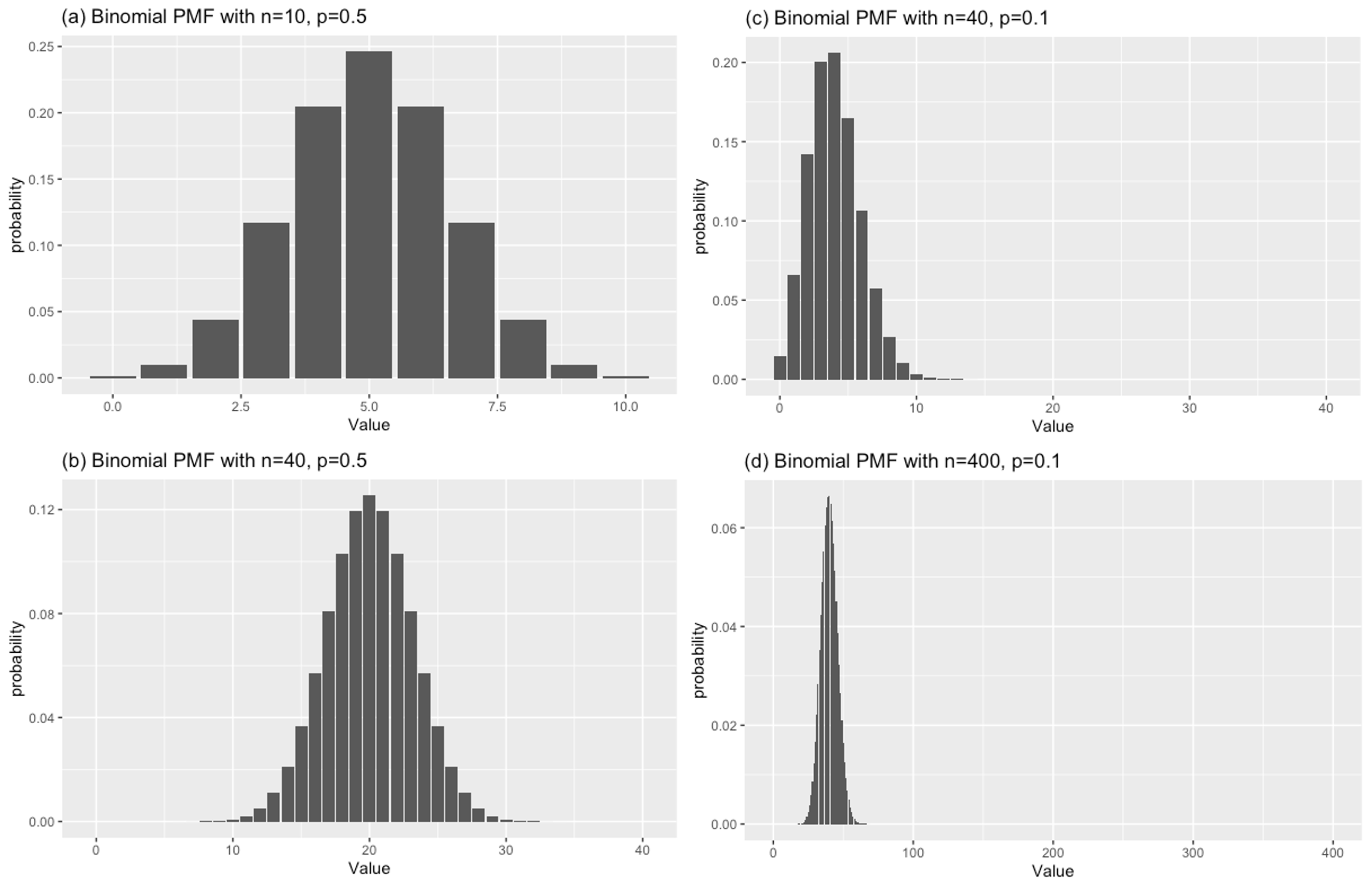
Fig. 7.7 Cases with different compatibilities with normal approximation
In Figure Fig. 7.7,
(a) is symmetric, but \(n\) is too small. It fails the rule-of-thumb tests. Normal approximation will not work well. ❌
(b) is symmetric with sufficiently large \(n\). It passes the rule-of-thumb tests. Normal approximation will work well. ✔
(c) has the same \(n\) as (b), but the distribution is very skewed because \(p=0.1\). Normal approximation will not work well. ❌
(d) has even larger \(n\) which compensates for the \(p\) far from 0.5. Normal approximation will work well.✔
7.4.3. Poisson Distribution and the CLT
A Poisson random variable counts the number of independent events occurring in a fixed interval, where events happen at a constant average rate \(\lambda\).
An interesting property of the Poisson distribution is that the sum of independent Poisson random variables is also Poisson distributed. If \(Y_1 \sim \text{Poisson}(\lambda_1)\) and \(Y_2 \sim \text{Poisson}(\lambda_2)\) are independent, then \(Y_1 + Y_2 \sim \text{Poisson}(\lambda_1 + \lambda_2)\).
By extension, if \(Y_1, Y_2, \cdots, Y_n\) are independent Poisson random variables with an identical rate parameter \(\lambda\), then:
Let \(X = \sum_{i=1}^n Y_i\) and \(\tilde{\lambda} = n\lambda\). Since \(Y_i\)’s are iid, the CLT applies for a sufficiently large \(n\):
Again, the normal parameters come from \(E[X]\) and \(\sigma_X\) of the true distribution.
When does it apply?
In practice, we do not have an explicit \(n\) for a Poisson random variable. If \(X \sim Pois(\lambda)\), it can be expressed as a sum of two Poisson random variables, each with parameter \(\lambda/2\), or of a thousand, each with parameter \(\lambda/1000\).
Thus we focus solely on the size of \(\lambda\). Typically, \(\lambda \geq 10\) is large enough for approximation by a normal distribution. See Fig. 7.8 to verify that the Poisson PMF grows more bell-shaped as \(\lambda\) becomes larger.
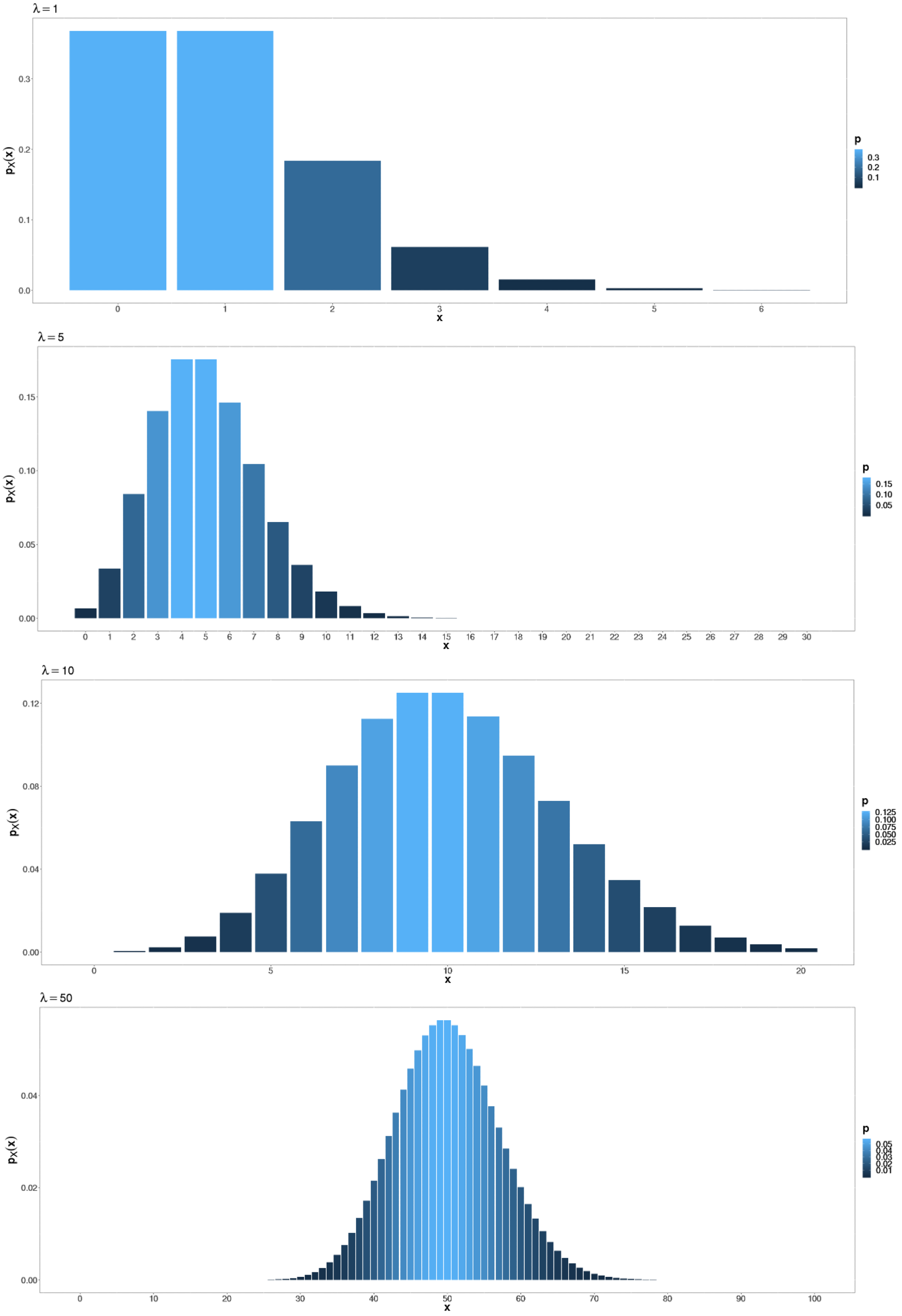
Fig. 7.8 \(\lambda =1,5,10,50\) from top to bottom, respectively.
7.4.4. The Practicality of Normal Approximation to Binomial & Poisson Distributions
Suppose a random variable \(X\) has a distribution \(B(n=100, p=0.5)\) and we are to compute \(P(X < 50)\). Without access to a computational software, we can either
compute \(P(X < 50)\) directly, which requires computation of 50 separate pmf terms: \(P(X=0) + P(X=1) + \cdots + P(X=49)\), or
use the approximate normal distribution to compute a slightly less accurate value in one access to the standard normal table.
As \(n\) gets larger, both the convenience and accuracy of Option 2 increase. This example only touches on the binomial case, but a similar logic can be applied to a Poisson case with a large \(\lambda\).
This technique was especially relevant when computational software was less accessible. Today, it still plays an important role in illustrating the broad implications of the CLT and in showing how different distributions are connected.
7.4.5. Continuity Correction
When using a normal distribution to approximate discrete distributions like the binomial or Poisson, we need to account for the difference between their supports. Consider \(X \sim B(n=100, p=0.5)\) again. Using the exact distribution,
But using its approximated distribution \(N(\mu=50, \sigma = \sqrt{25})\),
A discrete distribution always has a positive probability for a value in its support, while a normal distribution assigns a zero probability to any single value. This difference needs to be addressed by a technique called continuity correction, which is not covered in detail in this course. You are encouraged to read about it independently.
7.4.6. Bringing It All Together
Key Takeaways 📝
The CLT can be used to describe certain binomial and Poisson distributions.
For binomial distributions, the normal approximation works well when \(np \geq 10\) and \(n(1-p) \geq 10\) (or alternatively when \(np(1-p) \geq 10\)).
For Poisson distributions, the normal approximation works well when \(\lambda \geq 10\).
Continuity corrections may be needed when using a continuous distribution to approximate a discrete one.
7.4.7. Exercises
These exercises develop your skills in applying the Central Limit Theorem to approximate binomial and Poisson distributions with normal distributions.
Key Formulas
Normal Approximation to Binomial: If \(X \sim \text{Binomial}(n, p)\), then for large \(n\):
Rule of thumb: Approximation is adequate when \(np \geq 10\) and \(n(1-p) \geq 10\).
Normal Approximation to Poisson: If \(X \sim \text{Poisson}(\lambda)\), then for large \(\lambda\):
Rule of thumb: Approximation is adequate when \(\lambda \geq 10\).
Throughout these exercises, \(N(\mu, \sigma^2)\) denotes a normal distribution with mean \(\mu\) and variance \(\sigma^2\).
Note on Continuity Correction
When approximating a discrete distribution (binomial, Poisson) with a continuous normal distribution, continuity correction can improve accuracy by adjusting boundaries by ±0.5. For example, \(P(X \leq 45)\) for a discrete \(X\) would use \(P(Y \leq 45.5)\) in the normal approximation.
In this course, continuity correction is not required unless explicitly requested. Solutions below note where continuity correction would apply but compute answers without it for simplicity.
R Functions for Exact and Approximate Calculations
Exact binomial probabilities:
pbinom(x, size = n, prob = p)                # P(X ≤ x)
pbinom(x, size = n, prob = p, lower.tail = FALSE)  # P(X > x)
dbinom(x, size = n, prob = p)                # P(X = x)
Exact Poisson probabilities:
ppois(x, lambda)                             # P(X ≤ x)
ppois(x, lambda, lower.tail = FALSE)         # P(X > x)
dpois(x, lambda)                             # P(X = x)
Normal approximations:
# Binomial(n, p): use N(np, sqrt(np(1-p)))
mu <- n * p
sigma <- sqrt(n * p * (1 - p))
pnorm(x, mean = mu, sd = sigma)

# Poisson(λ): use N(λ, sqrt(λ))
pnorm(x, mean = lambda, sd = sqrt(lambda))
Exercise 1: Checking Approximation Conditions (Binomial)
For each binomial distribution, determine whether the normal approximation is appropriate. If so, state the approximate normal distribution.
\(X \sim \text{Binomial}(n = 200, p = 0.45)\)
\(X \sim \text{Binomial}(n = 50, p = 0.08)\)
\(X \sim \text{Binomial}(n = 80, p = 0.90)\)
\(X \sim \text{Binomial}(n = 500, p = 0.02)\)
\(X \sim \text{Binomial}(n = 30, p = 0.50)\)
Solution
For normal approximation to binomial, check: \(np \geq 10\) and \(n(1-p) \geq 10\).
Part (a): n = 200, p = 0.45
\(np = 200(0.45) = 90 \geq 10\) ✓
\(n(1-p) = 200(0.55) = 110 \geq 10\) ✓
Approximation is appropriate.
Part (b): n = 50, p = 0.08
\(np = 50(0.08) = 4 < 10\) ✗
Approximation is NOT appropriate. The expected number of successes is too small.
Part (c): n = 80, p = 0.90
\(np = 80(0.90) = 72 \geq 10\) ✓
\(n(1-p) = 80(0.10) = 8 < 10\) ✗
Approximation is NOT appropriate. The expected number of failures is too small.
Part (d): n = 500, p = 0.02
\(np = 500(0.02) = 10 \geq 10\) ✓ (borderline)
\(n(1-p) = 500(0.98) = 490 \geq 10\) ✓
Approximation is marginally appropriate (borderline at \(np = 10\)).
Note: With \(np\) exactly at the threshold, the approximation may be less accurate than for cases well above 10.
Part (e): n = 30, p = 0.50
\(np = 30(0.50) = 15 \geq 10\) ✓
\(n(1-p) = 30(0.50) = 15 \geq 10\) ✓
Approximation is appropriate.
Exercise 2: Normal Approximation to Binomial — Quality Control
A semiconductor manufacturing process has a 3% defect rate. In a batch of 400 chips:
Verify that the normal approximation to the binomial is appropriate.
Find the approximate probability that fewer than 10 chips are defective.
Find the approximate probability that between 10 and 20 chips (inclusive) are defective.
Find the approximate probability that more than 18 chips are defective.
Solution
Let \(X\) = number of defective chips, where \(X \sim \text{Binomial}(n = 400, p = 0.03)\).
Part (a): Check conditions
\(np = 400(0.03) = 12 \geq 10\) ✓
\(n(1-p) = 400(0.97) = 388 \geq 10\) ✓
Normal approximation is appropriate.
Parameters:
Part (b): P(X < 10)
“Fewer than 10” means \(X \leq 9\). Ignoring continuity correction:
Note: With continuity correction, we would use \(P(X \leq 9) \approx P(Z < 9.5)\), giving \(z = (9.5 - 12)/3.41 = -0.73\) and probability 0.2327, which is more accurate.
Part (c): P(10 ≤ X ≤ 20)
Ignoring continuity correction:
Note: With continuity correction, we would use boundaries 9.5 and 20.5.
Part (d): P(X > 18)
“More than 18” means \(X \geq 19\). Ignoring continuity correction:
Note: With continuity correction, we would use 18.5, giving \(z = 1.91\) and probability 0.0281.
R verification (exact vs. approximate):
n <- 400; p <- 0.03
mu <- n * p  # 12
sigma <- sqrt(n * p * (1 - p))  # 3.41

# Part (b): P(X < 10) = P(X ≤ 9)
pbinom(9, size = n, prob = p)              # Exact: 0.2384
pnorm(10, mean = mu, sd = sigma)           # Normal approx (no CC): 0.2789
pnorm(9.5, mean = mu, sd = sigma)          # Normal approx (with CC): 0.2327

# Part (c): P(10 ≤ X ≤ 20)
pbinom(20, n, p) - pbinom(9, n, p)         # Exact: 0.7240
pnorm(20, mu, sigma) - pnorm(10, mu, sigma) # Normal approx (no CC): 0.7029

# Part (d): P(X > 18) = P(X ≥ 19)
pbinom(18, n, p, lower.tail = FALSE)       # Exact: 0.0351
pnorm(18, mu, sigma, lower.tail = FALSE)   # Normal approx (no CC): 0.0393
Exercise 3: Checking Approximation Conditions (Poisson)
For each Poisson distribution, determine whether the normal approximation is appropriate. If so, state the approximate normal distribution.
\(X \sim \text{Poisson}(\lambda = 25)\)
\(X \sim \text{Poisson}(\lambda = 6)\)
\(X \sim \text{Poisson}(\lambda = 50)\)
A server receives requests at a rate of 3 per minute. Let \(X\) be the number of requests in a 5-minute window.
A call center receives calls at a rate of 0.5 per minute. Let \(X\) be the number of calls in an 8-hour shift.
Solution
For normal approximation to Poisson, check: \(\lambda \geq 10\).
Part (a): λ = 25
\(\lambda = 25 \geq 10\) ✓
Approximation is appropriate.
Part (b): λ = 6
\(\lambda = 6 < 10\) ✗
Approximation is NOT appropriate. Use exact Poisson calculations.
Part (c): λ = 50
\(\lambda = 50 \geq 10\) ✓
Approximation is appropriate.
Part (d): 3 requests/minute, 5-minute window
\(\lambda = 3 \times 5 = 15 \geq 10\) ✓
Approximation is appropriate.
Part (e): 0.5 calls/minute, 8-hour shift
8 hours = 480 minutes, so \(\lambda = 0.5 \times 480 = 240 \geq 10\) ✓
Approximation is appropriate (and highly accurate given the large \(\lambda\)).
Exercise 4: Normal Approximation to Poisson — Network Traffic
A network router receives packets at an average rate of 50 packets per second. Let \(X\) be the number of packets received in a 1-second interval.
What distribution does \(X\) follow? Verify that the normal approximation is appropriate.
Find the approximate probability that the router receives more than 60 packets in a second.
Find the approximate probability that the router receives between 40 and 55 packets (inclusive).
Find the value \(k\) such that \(P(X > k) \approx 0.05\).
Solution
Part (a): Distribution and conditions
\(X \sim \text{Poisson}(\lambda = 50)\).
Check: \(\lambda = 50 \geq 10\) ✓
Normal approximation is appropriate.
Part (b): P(X > 60)
“More than 60” means \(X \geq 61\). Ignoring continuity correction:
Note: With continuity correction (using 60.5), we get \(z = 1.48\) and probability 0.0694.
Part (c): P(40 ≤ X ≤ 55)
Ignoring continuity correction:
Note: With continuity correction (using 39.5 and 55.5), the probability would be slightly different.
Part (d): Find k such that P(X > k) ≈ 0.05
We need \(P(Z > z) = 0.05\), which gives \(z = z_{0.95} = 1.645\).
Ignoring continuity correction:
Since \(X\) takes integer values, \(P(X > 61) \approx 0.05\) or equivalently \(P(X \geq 62) \approx 0.05\).
Note: With continuity correction, we would solve for the boundary more precisely, but the integer threshold would be similar.
R verification (exact vs. approximate):
lambda <- 50
sigma <- sqrt(lambda)  # 7.07

# Part (b): P(X > 60)
ppois(60, lambda, lower.tail = FALSE)      # Exact: 0.0722
pnorm(60, mean = lambda, sd = sigma, lower.tail = FALSE)  # Normal approx: 0.0787

# Part (c): P(40 ≤ X ≤ 55)
ppois(55, lambda) - ppois(39, lambda)      # Exact: 0.7029
pnorm(55, lambda, sigma) - pnorm(40, lambda, sigma)  # Normal approx: 0.6818

# Part (d): Find k for P(X > k) ≈ 0.05
qnorm(0.95, mean = lambda, sd = sigma)     # Normal approx: 61.63
qpois(0.95, lambda)                        # Exact quantile: 62
Exercise 5: Comparing Approximation to Exact (Binomial)
Let \(X \sim \text{Binomial}(n = 100, p = 0.5)\).
Verify that the normal approximation is appropriate.
Using the normal approximation, find \(P(X \leq 45)\).
The exact probability is \(P(X \leq 45) = 0.1841\) (from software). How close is your approximation?
What feature of the binomial distribution (being discrete) causes the approximation error? How might “continuity correction” address this?
Solution
Part (a): Check conditions
\(np = 100(0.5) = 50 \geq 10\) ✓
\(n(1-p) = 100(0.5) = 50 \geq 10\) ✓
Normal approximation is appropriate.
Parameters:
Part (b): P(X ≤ 45) using normal approximation
Part (c): Comparison to exact
Exact: 0.1841
Approximation: 0.1587
Error: \(|0.1841 - 0.1587| = 0.0254\)
The approximation underestimates the true probability by about 0.025 (or about 14% relative error).
Part (d): Continuity correction
The binomial distribution is discrete—it assigns positive probability to each integer value. When we approximate with a continuous normal distribution, we’re replacing probability “bars” (each with width 1) with a smooth curve.
The issue: When computing \(P(X \leq 45)\) for the discrete binomial, we include the entire probability mass at \(X = 45\). But the normal approximation \(P(Z \leq -1.00)\) effectively “splits” this bar, capturing only the left half.
Continuity correction addresses this by adjusting boundaries by 0.5:
For \(P(X \leq 45)\), use \(P(X \leq 45.5)\) in the normal approximation
This gives \(z = (45.5 - 50)/5 = -0.90\), so \(P(Z \leq -0.90) = 0.1841\)
With continuity correction, the approximation matches the exact answer much more closely.
R verification:
n <- 100; p <- 0.5
mu <- n * p  # 50
sigma <- sqrt(n * p * (1 - p))  # 5

# Exact probability
pbinom(45, size = n, prob = p)
# [1] 0.1841

# Normal approximation (no continuity correction)
pnorm(45, mean = mu, sd = sigma)
# [1] 0.1587

# Normal approximation (with continuity correction)
pnorm(45.5, mean = mu, sd = sigma)
# [1] 0.1841
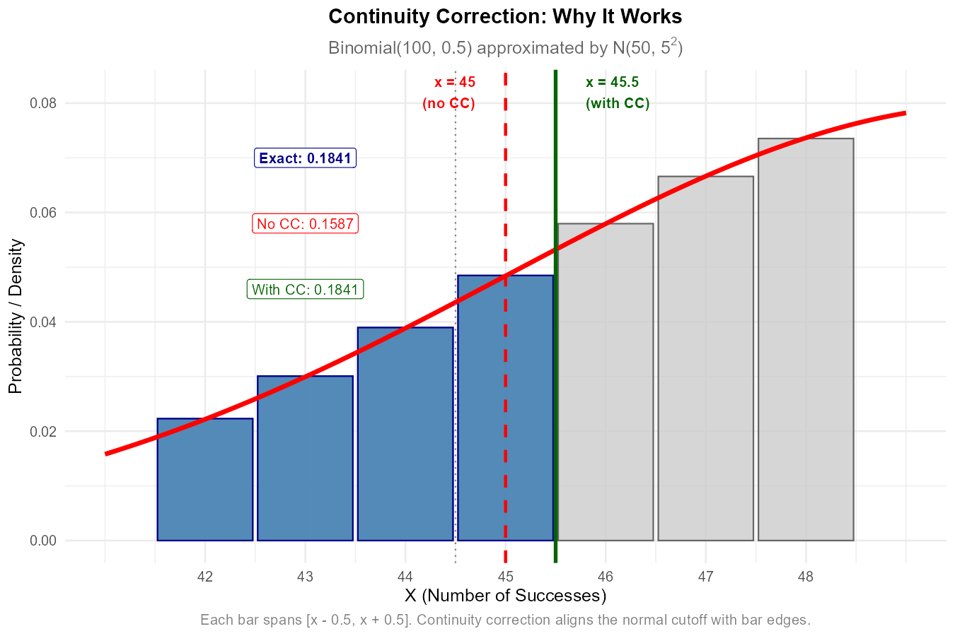
Fig. 7.9 Each binomial bar spans [x − 0.5, x + 0.5]. Continuity correction aligns the normal cutoff with bar edges.
Exercise 6: Why the CLT Applies
This exercise explores why the CLT leads to normal approximations for binomial and Poisson distributions.
A binomial random variable \(X \sim \text{Binomial}(n, p)\) can be written as \(X = \sum_{i=1}^{n} X_i\) where each \(X_i \sim \text{Bernoulli}(p)\). Explain why this representation allows us to apply the CLT.
For Bernoulli random variables with parameter \(p\):
What is \(E[X_i]\)?
What is \(\text{Var}(X_i)\)?
Use these to derive \(E[X]\) and \(\text{Var}(X)\) for \(X \sim \text{Binomial}(n, p)\).
Why does the condition “\(np \geq 10\) and \(n(1-p) \geq 10\)” make sense in terms of CLT convergence? (Hint: Think about the skewness of Bernoulli distributions for different \(p\) values.)
Explain why the normal approximation to the Poisson distribution improves as \(\lambda\) increases. (Hint: When \(\lambda\) is an integer, how can we express \(X \sim \text{Poisson}(\lambda)\) as a sum?)
Solution
Part (a): CLT for binomial
The representation \(X = \sum_{i=1}^{n} X_i\) expresses the binomial as a sum of \(n\) independent and identically distributed random variables (each \(X_i\) is Bernoulli(p)). The CLT applies to sums (or averages) of iid random variables with finite mean and variance. Since Bernoulli random variables have:
Finite mean: \(E[X_i] = p\)
Finite variance: \(\text{Var}(X_i) = p(1-p)\)
all CLT conditions are met. As \(n\) increases, the distribution of the sum approaches normal.
Part (b): Deriving binomial parameters from Bernoulli
For \(X_i \sim \text{Bernoulli}(p)\):
\(E[X_i] = p\)
\(\text{Var}(X_i) = p(1-p)\)
For \(X = \sum_{i=1}^{n} X_i\):
(The variance sum uses independence of the \(X_i\)’s.)
Part (c): Why np ≥ 10 and n(1-p) ≥ 10
The Bernoulli distribution is:
Symmetric when \(p = 0.5\)
Right-skewed when \(p < 0.5\) (more 0s than 1s)
Left-skewed when \(p > 0.5\) (more 1s than 0s)
The farther \(p\) is from 0.5, the more skewed each Bernoulli is, and the larger \(n\) must be for the CLT to produce a good normal approximation.
\(np \geq 10\) ensures enough expected successes so the right tail develops properly
\(n(1-p) \geq 10\) ensures enough expected failures so the left tail develops properly
Together, these conditions ensure the distribution has enough “room” on both sides to approximate a symmetric normal curve.
Part (d): CLT intuition for Poisson
When \(\lambda\) is a positive integer, we can write \(X \sim \text{Poisson}(\lambda)\) as a sum of \(\lambda\) independent \(\text{Poisson}(1)\) random variables:
Each \(Y_i\) has:
Mean: \(E[Y_i] = 1\)
Variance: \(\text{Var}(Y_i) = 1\)
As \(\lambda\) increases, we sum more iid terms, and CLT intuition suggests the distribution approaches normal. The variance of \(X\) equals \(\lambda\) (the number of terms), which grows with \(\lambda\).
The condition \(\lambda \geq 10\) ensures the Poisson has enough “spread” for an adequate normal approximation. Small \(\lambda\) produces highly right-skewed Poisson distributions concentrated near 0, similar to how small \(n\) produces poor CLT approximations for binomial.
Note: For non-integer \(\lambda\), this “sum of Poisson(1)” interpretation doesn’t apply exactly, but the intuition still holds—larger \(\lambda\) means more variability and a more symmetric, bell-shaped distribution.
Exercise 7: Application — Election Polling
A polling organization surveys 600 randomly selected voters. Suppose the true proportion supporting a candidate is \(p = 0.52\).
Let \(X\) be the number of supporters in the sample. What is the distribution of \(X\)?
Verify that the normal approximation is appropriate.
Find the approximate probability that fewer than 300 voters (less than 50%) support the candidate.
Find the approximate probability that the poll correctly identifies the candidate as having majority support (i.e., \(X > 300\)).
How would the probability in (d) change if the sample size were increased to 1500?
Solution
Part (a): Distribution
\(X \sim \text{Binomial}(n = 600, p = 0.52)\)
Part (b): Check conditions
\(np = 600(0.52) = 312 \geq 10\) ✓
\(n(1-p) = 600(0.48) = 288 \geq 10\) ✓
Normal approximation is appropriate.
Parameters:
Part (c): P(X < 300)
“Fewer than 300” means \(X \leq 299\). Ignoring continuity correction:
There is about a 16.4% chance that the poll shows fewer than 50% support, even though the true support is 52%.
Note: With continuity correction (using 299.5), the probability would be slightly different.
Part (d): P(X > 300)
“More than 300” means \(X \geq 301\). Ignoring continuity correction:
There is about an 83.7% chance that the poll correctly identifies majority support.
Part (e): Effect of increasing n to 1500
With \(n = 1500\):
\(P(X > 750)\) (ignoring continuity correction):
With \(n = 1500\), there is about a 93.9% chance of correctly identifying majority support—a significant improvement from 83.7%.
Key insight: Larger samples produce more precise estimates, reducing the probability of incorrect conclusions.
R verification:
# n = 600
n <- 600; p <- 0.52
mu <- n * p  # 312
sigma <- sqrt(n * p * (1 - p))  # 12.24

# Part (c): P(X < 300)
pbinom(299, n, p)                           # Exact: 0.1612
pnorm(300, mean = mu, sd = sigma)           # Normal approx: 0.1635

# Part (d): P(X > 300)
pbinom(300, n, p, lower.tail = FALSE)       # Exact: 0.8264
pnorm(300, mu, sigma, lower.tail = FALSE)   # Normal approx: 0.8365

# Part (e): n = 1500
n2 <- 1500
mu2 <- n2 * p  # 780
sigma2 <- sqrt(n2 * p * (1 - p))  # 19.35
pnorm(750, mu2, sigma2, lower.tail = FALSE) # 0.9393
Exercise 8: Application — Server Reliability
A data center monitors server errors. On average, critical errors occur at a rate of 2 per hour.
What is the distribution of \(X\), the number of critical errors in a 12-hour period?
Is the normal approximation appropriate? If so, state the approximate distribution.
Find the approximate probability of more than 30 errors in a 12-hour period.
The data center triggers an alert if the error count exceeds a threshold \(k\). Find \(k\) such that alerts occur approximately 1% of the time under normal operating conditions.
If the error rate doubles (to 4 per hour) due to a problem, what is the probability of triggering an alert at the threshold from (d)?
Solution
Part (a): Distribution
Errors occur at rate 2 per hour. In 12 hours:
\(\lambda = 2 \times 12 = 24\)
\(X \sim \text{Poisson}(24)\)
Part (b): Normal approximation check
\(\lambda = 24 \geq 10\) ✓
Normal approximation is appropriate.
Part (c): P(X > 30)
“More than 30” means \(X \geq 31\). Ignoring continuity correction:
About 11% probability of more than 30 errors.
Note: With continuity correction (using 30.5), \(z = 1.33\) and probability ≈ 0.092.
Part (d): Find k for 1% alert rate
We need \(P(X > k) = 0.01\), so \(P(X \leq k) = 0.99\).
From Z-table: \(z_{0.99} = 2.33\).
Ignoring continuity correction:
Since \(X\) is discrete, set threshold at \(k = 35\). Alert triggers when \(X > 35\) (i.e., \(X \geq 36\)), which occurs approximately 1% of the time.
Part (e): Detection probability when rate doubles
If rate = 4 per hour, then \(\lambda = 4 \times 12 = 48\) for 12 hours.
Probability of alert (\(X > 35\)), ignoring continuity correction:
There is about a 97% probability of detecting the doubled error rate—the alerting system is effective at identifying the problem.
R verification:
# Normal operating conditions: λ = 24
lambda1 <- 24
sigma1 <- sqrt(lambda1)  # 4.90

# Part (c): P(X > 30)
ppois(30, lambda1, lower.tail = FALSE)      # Exact: 0.0958
pnorm(30, lambda1, sigma1, lower.tail = FALSE)  # Normal approx: 0.1103

# Part (d): Find k for 1% alert rate
qpois(0.99, lambda1)                        # Exact: 36
qnorm(0.99, lambda1, sigma1)                # Normal approx: 35.39

# Part (e): Problem conditions: λ = 48
lambda2 <- 48
sigma2 <- sqrt(lambda2)  # 6.93

# Detection probability with k = 35
ppois(35, lambda2, lower.tail = FALSE)      # Exact: 0.9691
pnorm(35, lambda2, sigma2, lower.tail = FALSE)  # Normal approx: 0.9696
7.4.8. Additional Practice Problems
True/False Questions (1 point each)
The normal approximation to a binomial distribution requires only that \(n\) be large.
Ⓣ or Ⓕ
If \(X \sim \text{Poisson}(\lambda = 5)\), the normal approximation is appropriate.
Ⓣ or Ⓕ
For \(X \sim \text{Binomial}(n = 100, p = 0.95)\), the normal approximation is appropriate.
Ⓣ or Ⓕ
The variance of the normal approximation to \(\text{Poisson}(\lambda)\) equals \(\lambda\).
Ⓣ or Ⓕ
Continuity correction is needed because the binomial and Poisson are discrete, while the normal is continuous.
Ⓣ or Ⓕ
The sum of independent Poisson random variables is also Poisson distributed.
Ⓣ or Ⓕ
Multiple Choice Questions (2 points each)
For \(X \sim \text{Binomial}(n = 200, p = 0.3)\), the normal approximation is \(N(\mu, \sigma^2)\) with:
Ⓐ \(\mu = 60, \sigma^2 = 42\)
Ⓑ \(\mu = 60, \sigma^2 = 18\)
Ⓒ \(\mu = 0.3, \sigma^2 = 42\)
Ⓓ \(\mu = 200, \sigma^2 = 60\)
Which binomial distribution can be approximated well by a normal distribution?
Ⓐ \(\text{Binomial}(n = 20, p = 0.5)\)
Ⓑ \(\text{Binomial}(n = 100, p = 0.02)\)
Ⓒ \(\text{Binomial}(n = 50, p = 0.3)\)
Ⓓ \(\text{Binomial}(n = 200, p = 0.98)\)
For \(X \sim \text{Poisson}(\lambda = 36)\), find \(P(X > 42)\) using the normal approximation (ignoring continuity correction):
Ⓐ \(P(Z > 0.5)\)
Ⓑ \(P(Z > 1.0)\)
Ⓒ \(P(Z > 6.0)\)
Ⓓ \(P(Z > 1.17)\)
The normal approximation to binomial works better when:
Ⓐ \(p\) is close to 0 or 1
Ⓑ \(n\) is small
Ⓒ \(p\) is close to 0.5
Ⓓ \(np < 10\)
If \(Y_1 \sim \text{Poisson}(8)\) and \(Y_2 \sim \text{Poisson}(12)\) are independent, then \(Y_1 + Y_2 \sim\):
Ⓐ \(\text{Poisson}(96)\)
Ⓑ \(\text{Poisson}(20)\)
Ⓒ \(\text{Binomial}(20, 0.5)\)
Ⓓ \(N(20, 20)\)
For the normal approximation to \(\text{Binomial}(n, p)\), both \(np \geq 10\) and \(n(1-p) \geq 10\) are required because:
Ⓐ The CLT requires at least 20 observations
Ⓑ These ensure sufficient expected successes and failures for symmetry
Ⓒ The binomial variance must exceed 10
Ⓓ The normal distribution requires integer parameters
Answers to Practice Problems
True/False Answers:
False — Both \(n\) and \(p\) matter. We need \(np \geq 10\) and \(n(1-p) \geq 10\).
False — \(\lambda = 5 < 10\), so the normal approximation is not appropriate.
False — \(n(1-p) = 100(0.05) = 5 < 10\), so the condition fails.
True — For Poisson(\(\lambda\)), both the mean and variance equal \(\lambda\), so the normal approximation has variance \(\lambda\).
True — The discrete-to-continuous mismatch causes approximation error, which continuity correction helps address.
True — If \(Y_1 \sim \text{Poisson}(\lambda_1)\) and \(Y_2 \sim \text{Poisson}(\lambda_2)\) are independent, then \(Y_1 + Y_2 \sim \text{Poisson}(\lambda_1 + \lambda_2)\).
Multiple Choice Answers:
Ⓐ — \(\mu = np = 200(0.3) = 60\); \(\sigma^2 = np(1-p) = 200(0.3)(0.7) = 42\).
Ⓒ — Check each: (A) \(np = 10\), \(n(1-p) = 10\) — borderline; (B) \(np = 2 < 10\) — fails; (C) \(np = 15 \geq 10\), \(n(1-p) = 35 \geq 10\) — passes well; (D) \(n(1-p) = 4 < 10\) — fails.
Ⓑ — \(\sigma = \sqrt{36} = 6\); ignoring continuity correction, \(z = (42 - 36)/6 = 1.0\).
Ⓒ — When \(p \approx 0.5\), the Bernoulli distribution is symmetric, so the CLT converges faster.
Ⓑ — Sum of independent Poissons is Poisson with \(\lambda = 8 + 12 = 20\). (Note: The normal approximation N(20, 20) could be used since \(\lambda = 20 \geq 10\), but the exact distribution is Poisson(20).)
Ⓑ — These conditions ensure enough expected successes (np) and failures (n(1-p)) so the distribution has adequate spread on both sides to resemble a symmetric bell curve.