Slides 📊

• Hypothesis Testing for Single Sample (Part 2) (PPTX)

10.2. Hypothesis Test for the Population Mean When σ is Known

In the previous lesson, we learned the conceptual framework of hypothesis testing and constructed a simple rule for rejecting the null hypothesis in an upper-tailed test. Let us now extend this concept to all three types of hypotheses (upper-tailed, lower-tailed, and two-tailed), and discuss an alternative decision-making method using p-values.

Road Map 🧭

• Organize the formal hypothesis pairs and decision rules for the three types of tests on a population mean (upper-tailed, lower-tailed, and two-tailed), when \(\sigma\) is known.

• Learn the p-value method for making decisions and compare it with the cutoff method.

10.2.1. Z-Test for Population Means

Summary of the Three Dual Hypotheses

In Section 10.1.1, we learned how to translate a research question about a population mean into a pair of formal hypotheses. Such pairs take three general forms, whose properties are summarized in the table below:

Name of test	Hypotheses	Question
Upper-tailed (right-tailed)	\[\begin{split}&H_0: \mu \leq \mu_0\\ &H_a: \mu > \mu_0\end{split}\]	The population mean \(\mu\) is suspected to be greater than a baseline belief, \(\mu_0\)
Lower-tailed (left-tailed)	\[\begin{split}&H_0: \mu \geq \mu_0\\ &H_a: \mu < \mu_0\end{split}\]	The population mean \(\mu\) is suspected to be less than a baseline belief, \(\mu_0\)
Two-tailed	\[\begin{split}&H_0: \mu = \mu_0\\ &H_a: \mu \neq \mu_0\end{split}\]	The population mean \(\mu\) is suspected to be different than a baseline belief, \(\mu_0\)

The Assumptions

Recall the assumptions needed for the decision-rule construction in Section 10.1.1:

1. \(X_1, X_2, \cdots, X_n\) form an iid sample from the population \(X\) with mean \(\mu\) and variance \(\sigma^2\).

2. Either the population \(X\) is normally distributed, or the sample size \(n\) is sufficiently large for the CLT to hold.

3. The population variance \(\sigma^2\) is known.

These assumptions allowed us to use the CLT to establish:

\[\bar{X} \sim N\left(\mu_0, \frac{\sigma}{\sqrt{n}}\right)\]

under the null hypothesis. The distributional property of \(\bar{X}\) continues to play a crucial role for the remaining two decision rules.

The Decision Rules

A. Upper-Tailed Hypothesis Test — A Review

In an upper-tailed hypothesis test, with

\[\begin{split}&H_0: \mu \leq \mu_0\\ &H_a: \mu > \mu_0,\end{split}\]

we agreed to reject the null hypothesis when the observed sample mean was too large to be a typical value under the null haypothesis.

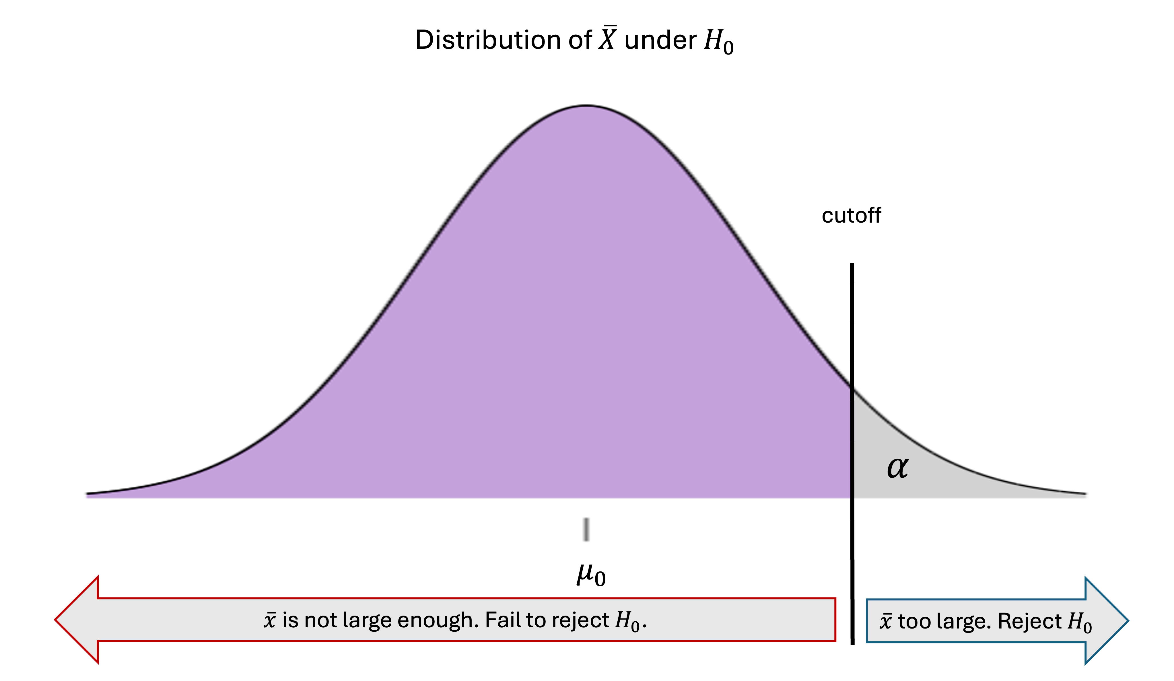
Fig. 10.12 Decision rule for upper-tailed hypothesis test

Specifically, we reject \(H_0\) when \(\bar{x}\) is on the upper \(\alpha\cdot100\)-th percentile of the null distribution:

\[\bar{x} > \text{cutoff}_{upper} = z_\alpha\frac{\sigma}{\sqrt{n}} +\mu_0.\]

By standardizing both sides of the inequality, the null hypothesis is rejected when:

\[\frac{\bar{x}-\mu_0}{\sigma/\sqrt{n}} > z_\alpha.\]

B. Lower-Tailed Hypthesis Test — A Mirror Argument

Recall the pair of hypotheses for a lower-tailed test:

\[\begin{split}&H_0: \mu \geq \mu_0\\ &H_a: \mu < \mu_0.\end{split}\]

The rule for rejecting the null hypothesis follows the same chain of logic as the upper-tailed case, only with the sides flipped. Since we are now challenging the status quo belief that \(H_0:\mu \geq \mu_0\), we must reject the null hypothesis if the evidence from the sample mean is too low.

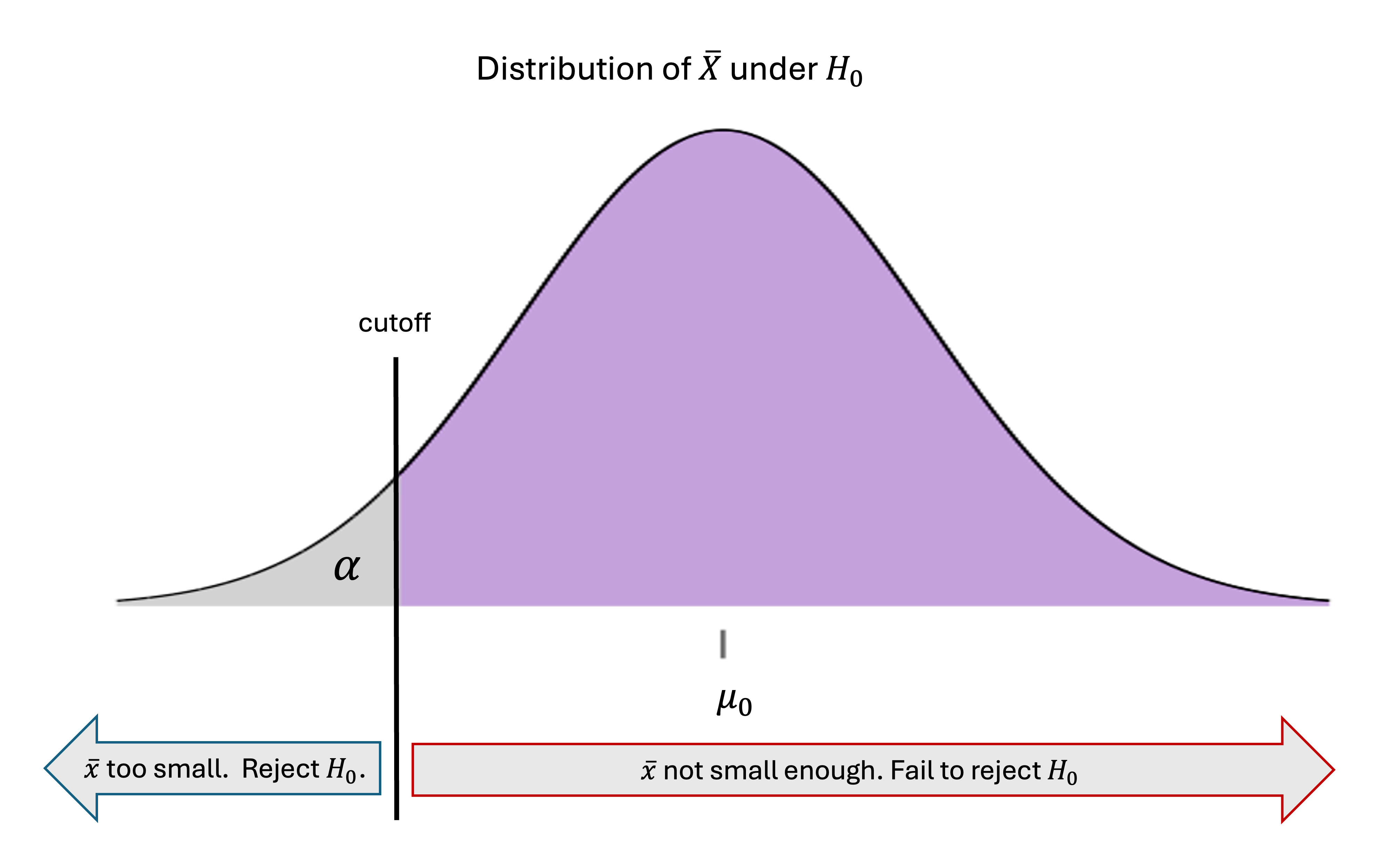
Fig. 10.13 Decision rule for lower-tailed hypothesis test

Formally, the null hypothesis is rejected if the observed sample mean falls below the lower \(\alpha \cdot 100\)-th percentile of the null distribution, or if \(\bar{x} < -z_\alpha\frac{\sigma}{\sqrt{n}} + \mu_0\). Standardizing both sides, rejection occurs when:

\[\frac{\bar{x}-\mu_0}{\sigma/\sqrt{n}} < -z_\alpha.\]

C. Two-Tailed Hypothesis Test — Splitting the Error Probability in Half

In a two-tailed hypothesis test with

\[\begin{split}&H_0: \mu = \mu_0\\ &H_a: \mu \neq \mu_0,\end{split}\]

we are starting off with the belief that the true mean is equal to \(\mu_0\). Thus, an extreme deviation on either side should lead to its rejection. We set two cutoffs—upper and lower—around \(\mu_0\) and reject the null if the sample mean falls outside this range by being either too small or too large.

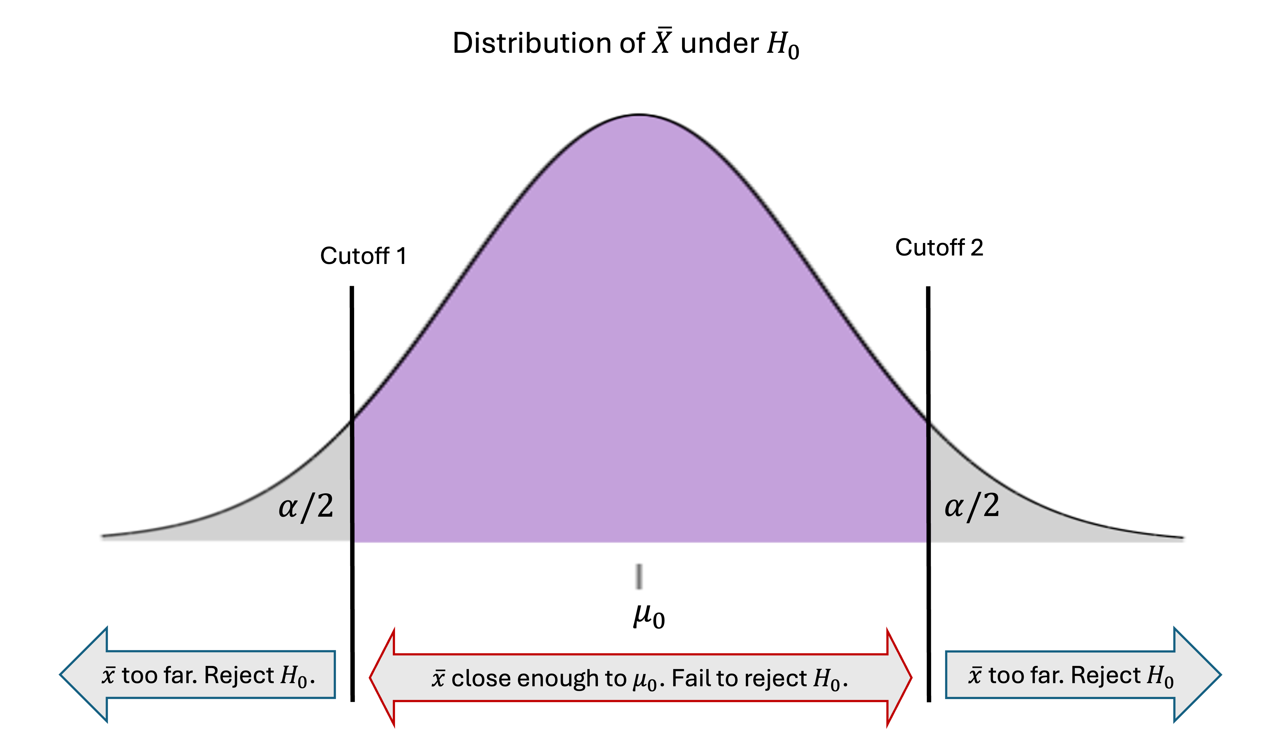
Fig. 10.14 Decision rule for two-tailed hypothesis test

To identify rejection regions on both ends of the null distribution while keeping the Type I error probability to at most \(\alpha\), we must split \(\alpha\) into half for each tail. \(H_0\) is rejected either if

\[\bar{x} > z_{\alpha/2}\frac{\sigma}{\sqrt{n}} + \mu_0 \quad \text{ or if } \quad \bar{x} < -z_{\alpha/2}\frac{\sigma}{\sqrt{n}} + \mu_0.\]

By standardizing both sides and combining the two cases using an absolute value sign, this rule is equivalent to rejecting the null when:

\[\left|\frac{\bar{x}-\mu_0}{\sigma/\sqrt{n}}\right| > z_{\alpha/2}.\]

10.2.2. The \(p\)-Value Method

While we could use cutoffs and rejection regions to draw conclusions to a hypothesis test, the convention is to use an alternative \(p\)-value method. We will learn that this method provides more nuanced information about the strength of evidence against the null hypothesis.

What Is the \(p\)-Value Method?

The \(p\)-value method focuses on the tail area created by the observed sample mean instead of its \(x\)-axis location on the null distribution. Let us use an upper-tailed case for our initial illustration:

\[\begin{split}& H_0: \mu \leq \mu_0\\ & H_0: \mu > \mu_0\end{split}\]

First, suppose we observe \(\bar{x}\) that is too large for the null and falls in the rejection region. The tail area created by \(\bar{x}\), marked in blue in Fig. 10.15, is bound to be smaller than \(\alpha\).

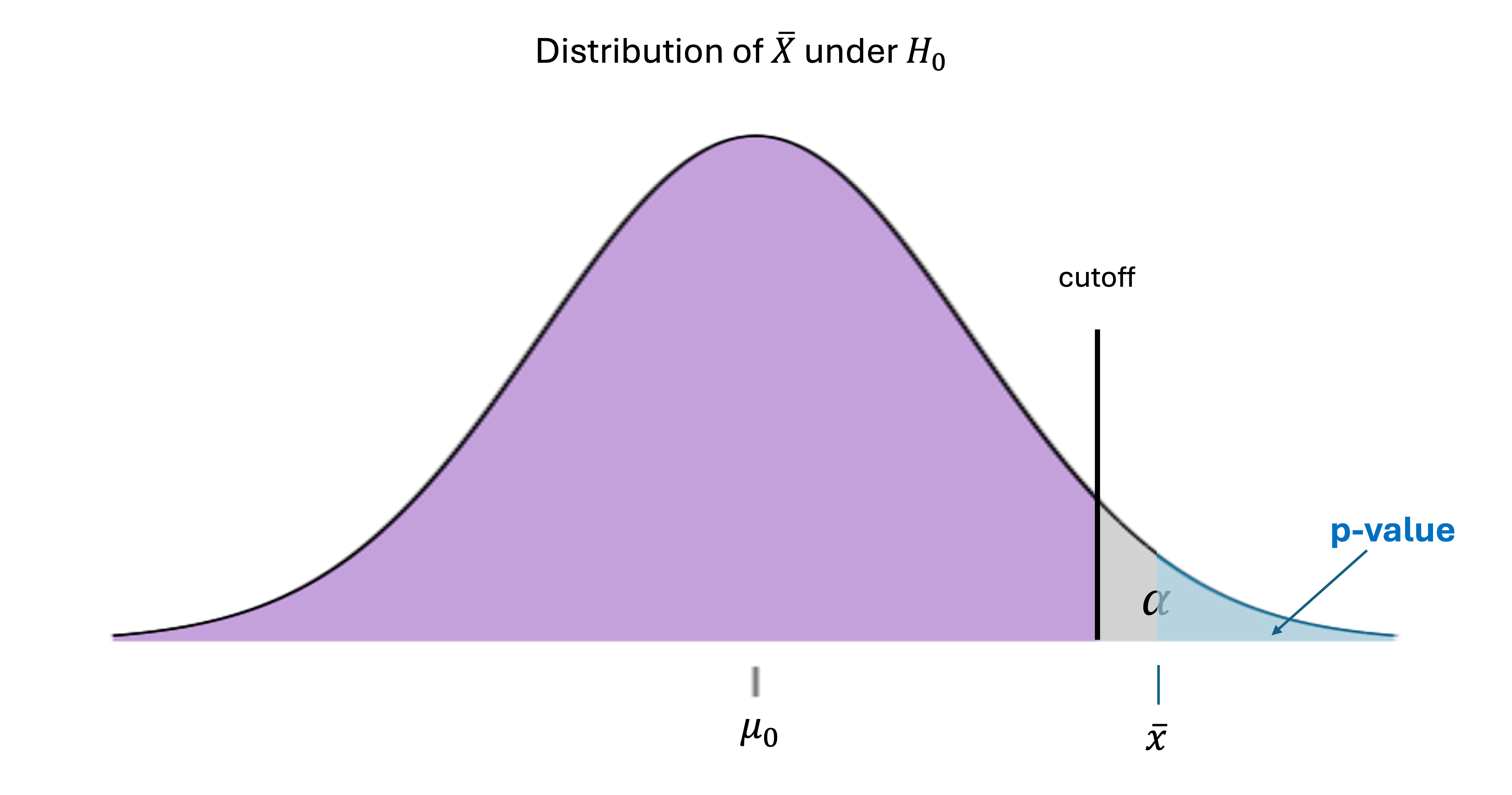
Fig. 10.15 P-value when the null hypothesis is rejected (upper-tailed test)

Let us also observe a case where \(\bar{x}\) is not large enough to be rejected. We find that the tail area created by \(\bar{x}\) must be at least of size \(\alpha\).

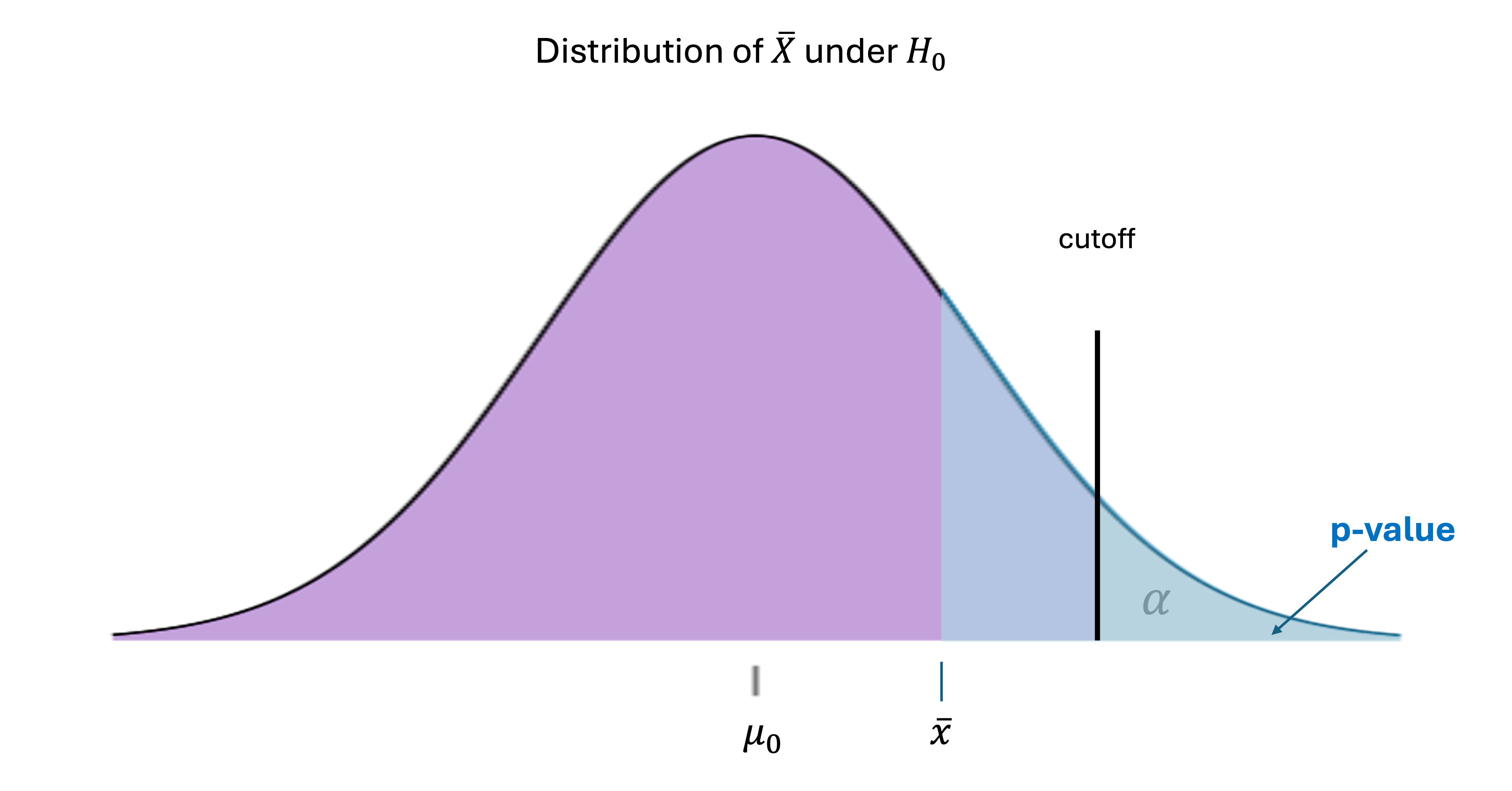
Fig. 10.16 P-value when the null hypothesis is not rejected (upper-tailed test)

The takeaway here is that comparing p-values againt \(\alpha\) can be used as an alternative to comparing \(z_{TS}\) against a \(z\)-critical value for a conclusion. We will define \(p\)-values for the remaining two test types so that in every case, a \(p\)-value smaller than \(\alpha\) leads to the rejection of \(H_0\).

How To Compute \(p\)-Values

A \(p\)-value is universally interpreted as “the probability of observing an outcome at least as unusual as the current one, under the null hypothesis”. Let us first confirm that the upper-tailed \(p\)-value explored in the previous section agrees with this general description. We will then define \(p\)-values for the remaining test types accordingly.

A. \(p\)-Value for an Upper-Tailed Hypothesis Test

We translate the general description of \(p\)-values to a mathematical expression for an upper-tailed hypothesis test:

\[p\text{-value} = P(\bar{X} \geq \bar{x} |H_0 \text{ is true}).\]

This setup aligns with the graphical illustrations in Fig. 10.15 and Fig. 10.16, as well as the description in words. If it is believed that \(\mu\) is less than or equal to a value, the “unsual” case would always correspond to the larger side. Let us continue to simplify the \(p\)-value:

\[\begin{split}p\text{-value} &= P(\bar{X} \geq \bar{x} |H_0 \text{ is true})\\ &=P\left(\frac{\bar{X}-\mu_0}{\sigma/\sqrt{n}} \geq \frac{\bar{x}-\mu_0}{\sigma/\sqrt{n}} \Bigg|H_0 \text{ is true}\right)\\ &=P(Z \geq z_{TS})\end{split}\]

This can be computed in R using:

zts <- (xbar - mu0)/(sigma/sqrt(n))
pvalue <- pnorm(zts, lower.tail=FALSE)

B. \(p\)-Value for a Lower-Tailed Hypothesis Test

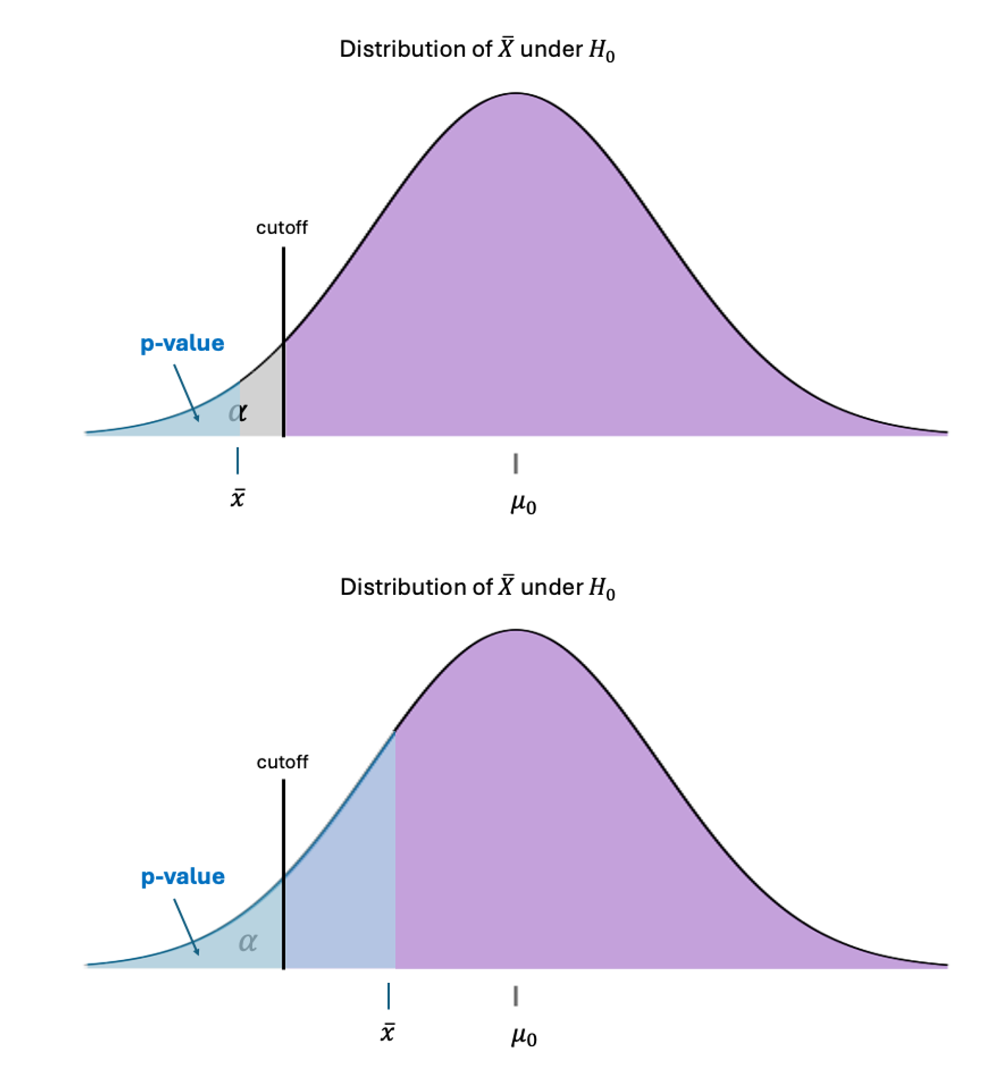
Fig. 10.17 Upper: \(p\)-value when \(\bar{x}\) is in the rejection region; Lower: \(p\)-value when \(\bar{x}\) is not small enough

In a lower-tailed hypothesis test where the baseline belief is that \(\mu\) is greater than or equal to a \(\mu_0\), the “unusual” is always toward the lower end.

\[\begin{split}\text{p-value} &= P(\bar{X} \leq \bar{x}|H_0 \text{ is true})\\ &=P\left(\frac{\bar{X}-\mu_0}{\sigma/\sqrt{n}} \leq \frac{\bar{x}-\mu_0}{\sigma/\sqrt{n}} \Bigg|H_0 \text{ is true}\right)\\ &=P(Z \leq z_{TS})\end{split}\]

zts <- (xbar - mu0)/(sigma/sqrt(n))
pvalue <- pnorm(zts)

C. \(p\)-Value for a Two-Tailed Hypothesis Test

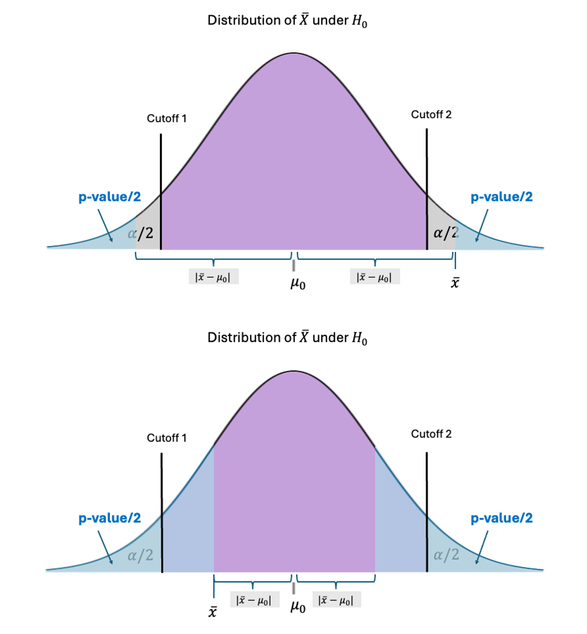
Fig. 10.18 Upper: \(p\)-value when \(\bar{x}\) is in the rejection region; Lower: \(p\)-value when \(\bar{x}\) is not far enough from \(\mu_0\)

In a two-tailed hypothesis test, we must consider the “unusual” deviations on both sides. Therefore, we compute the area corresponding to larger absolute deviations from \(\mu_0\) than the currently observed \(|\bar{x}-\mu_0|\):

\[\text{p-value} = P(|\bar{X}-\mu_0|\geq |\bar{x}-\mu_0| \big| H_0 \text{ is true})\]

Dividing both sides of the inequality by the standard error \(\sigma/\sqrt{n}\),

\[\begin{split}\text{p-value} &= \left(\frac{|\bar{X}-\mu_0|}{\sigma/\sqrt{n}}\geq \frac{|\bar{x}-\mu_0|}{\sigma/\sqrt{n}} \Bigg| H_0 \text{ is true} \right)\\ &= P(|Z| \geq |z_{TS}|)\\ &= P(Z \leq -|z_{TS}| \text{ or } Z \geq |z_{TS}|) \\ &=2P(Z \leq -|z_{TS}|) = 2P(Z \geq |z_{TS}|)\\\end{split}\]

The final two steps are true due to the symmetry of the standard normal distribution around \(0\). Either can be used for computation.

abs_zts <- abs((xbar - mu0)/(sigma/sqrt(n)))
pvalue <- 2 * pnorm(-abs_zts)

#alternatively,
pvalue <- 2 * pnorm(abs_zts, lower.tail=FALSE)

Making the Decision

Once the \(p\)-value is obtained, we compare it to the pre-specified significance level \(\alpha\).

• If \(p\)-value \(< \alpha\), reject \(H_0\).

• If \(p\)-value \(\geq \alpha\), fail to reject \(H_0\).

Why is the \(p\)-Value Method Preferred?

The \(p\)-value method is generally preferred over the cutoff method for two main reasons.

1. Its decision rule does not depend on the test type. A small \(p\)-value always indicates evidence against the null hypothesis, whether the test is lower-tailed, upper-tailed, or two-tailed.

2. More importantly, it conveys the strength of the data evidence without referencing a fixed standard, \(\alpha\). Whether \(\alpha=0.05\) or \(\alpha=0.01\), a \(p\)-value of \(0.00001\) universally implies a very strong evidence against the null, while a \(p\)-value of \(0.9\) indicates little or no of evidence.

   Because a \(p\)-value lies in \([0,1]\), we also have a more natural intuition for its size, compared with the test statistic \(z_{TS}\), which can in principle take any real value.

Example 💡: Spiral Galaxy Diameters

A theory predicts that spiral galaxies have an average diameter of 50,000 light years. A research group wants to test whether local galaxies in a neighborhood of Milky Way are larger than this overall average using \(\alpha = 0.01\).

• The study has an SRS of 50 spiral galaxies from a catalog.

• Their sample mean is \(\bar{x} = 51,600\) light years.

• The population standard deviation is known to be \(\sigma = 4,000\) light years.

• The data appears fairly symmetric and is free of outliers.

Step 0: Check Assumptions

The data does not have a strong deviation from normality and the sample is an SRS from the population, so the sample size of 50 is large enough for CLT to hold. Since the population standard deviation is known, our use of the \(z\)-test procedure is justified.

Step 1: Define the Parameter

Let \(\mu\) represent the true mean diameter of spiral galaxies in the chosen neighborhood of Milky Way.

Step 2: State the Hypothesis

• \(H_0: \mu \leq 50,000\)

• \(H_a: \mu > 50,000\)

Step 3: Calculate the Observed Test Statistic and the P-Value

\[z_{TS} = \frac{\bar{x} - \mu_0}{\sigma/\sqrt{n}} = \frac{51,600 - 50,000}{4,000/\sqrt{50}} = \frac{1,600}{565.685} = 2.828\]

Since this is a right-tailed test,

zts <- 2.828
p_value <- pnorm(zts, lower.tail = FALSE)
p_value
# [1] 0.002339

Step 4: Make the Decision and State the Conclusion

Since \(p\)-value \(=0.002339 < 0.01\) we reject the null hypothesis. With the significance level \(\alpha=0.01\), we have sufficient evidence that the true mean diameter of spiral galaxies in this neighborhood is greater than 50,000 light years.

🔎 See the Appendix at the end of this lession for additional practice on power and sample size computation in the same context.

Example 💡: A Manufacturing Quality Control

Bulls Eye Production manufactures precision components whose diameters follow a normal distribution with mean 5mm and standard deviation 0.5mm. The company collects a random sample as part of their regular maintenance. If the sample provides evidence that the true mean diameter differs significantly from 5mm, they must recaibrate the production equipment. From the previous round of the regular maintenance, the company obtained the following result:

• Sample size: \(n = 64\)

• Sample mean: \(\bar{x} = 4.85\) mm

• Population standard deviation: \(\sigma = 0.5\) mm

• Significance level: \(\alpha = 0.01\)

Step 0: Can We Use a \(z\)-Test?

The population distribution is known to be normal, which guarantees that its sample mean will be normally distributed for any sample size. \(n=64\) is large enough even if the population has moderate deviations from normal. Since the population standard deviation is also known, we have enough justification to use a \(z\)-test procedure.

Step 1: Define the Parameter

Let us use \(\mu\) to denote the true mean diamter of the components produced by the current production equipment.

Step 2: State the Hypotheses

\[\begin{split}&H_0: \mu = 5\\ &H_a: \mu \neq 5\end{split}\]

Step 2: Calculate the Observed Test Statistic and the P-Value

\[Z_{TS} = \frac{\bar{x} - \mu_0}{\sigma/\sqrt{n}} = \frac{4.85 - 5.0}{0.5/\sqrt{64}} = \frac{-0.15}{0.0625} = -2.4\]

For a two-tailed test, we need the probability of observing a test statistic at least as extreme as \(\pm 2.4\):

z_test_stat <- -2.4
p_value <- 2 * pnorm(abs(z_test_stat), lower.tail = FALSE)
p_value
# [1] 0.01639472

Step 4: Make the Decision and Write the Conclusion

• p-value \(= 0.0164\)

• \(\alpha = 0.01\)

Since \(0.0164 > 0.01\), we fail to reject the null hypothesis. At the 1% significance level, we do not have sufficient evidence to conclude that the population mean of component diameters is different than 5mm.

10.2.3. Bringing It All together

Key Takeaways 📝

1. \(z\)-tests for population means are used when the population standard deviation is known and the sampling distribution of the sample mean can be approximated with normal using the CLT.

2. The test statistic \(Z_{TS} = \frac{\bar{X} - \mu_0}{\sigma/\sqrt{n}}\) provides standardized evidence against the null hypothesis.

3. A \(p\)-value quantifies the strength of data evidence by providing the probability of observing more unusual results than the current one under the null hypothesis.

Exercises

1. Pharmaceutical Testing: A pharmaceutical company claims their new pain medication reduces recovery time from an average of 7.2 days to less than that. In a clinical trial of 100 patients, the sample mean recovery time was 6.8 days. Assuming \(\sigma = 1.5\) days, test the company’s claim at \(\alpha = 0.05\).

2. Manufacturing: A bottling company targets 12 oz per bottle. Quality control samples 36 bottles and finds \(\bar{x} = 11.85\) oz. With \(\sigma = 0.6\) oz, test whether the process mean differs from target at \(\alpha = 0.02\).

3. \(p\)-Value Interpretation: A study reports a \(p\)-value of 0.08 for testing \(H_0: \mu = 100\) versus \(H_a: \mu \neq 100\). Write three different statements about what this \(p\)-value means, avoiding common misinterpretations.

10.2.4. Appendix: Power Analysis for the Galaxy Study

Example 💡: Compute Power for the Galaxy Study

Suppose the researchers want to know their power to detect galaxies that are 2,000 light years larger on average than the theory predicts (i.e., \(\mu_a = 52,000\) light years).

Step 1: Find the Critical Cutoff Value

Under the null hypothesis, we reject \(H_0\) when our test statistic exceeds \(z_{0.01} = 2.326\):

z_alpha <- qnorm(0.01, lower.tail = FALSE)
z_alpha
# [1] 2.326348

The corresponding cutoff value for \(\bar{x}\) is:

\[\bar{x}_{cutoff} = \mu_0 + z_{\alpha} \cdot \frac{\sigma}{\sqrt{n}} = 50,000 + 2.326 \times \frac{4,000}{\sqrt{50}} = 51,316\]

Step 2: Calculate Type II Error Probability

If the true mean is \(\mu_a = 52,000\), the Type II error is the probability that \(\bar{X} < 51,316\):

# Type II error calculation
beta <- pnorm(51316, mean = 52000, sd = 4000/sqrt(50), lower.tail = TRUE)
beta
# [1] 0.1132957

Step 3: Calculate Power

\[\text{Power} = 1 - \beta = 1 - 0.113 = 0.887\]

Interpretation

This study has about 88.7% power to detect a 2,000 light-year increase in galaxy diameter. This is quite good power—if galaxies in this region truly average 52,000 light years in diameter, there’s about an 89% chance this study would detect that difference.

Example 💡: Compute the Required Sample Size for the Galaxy Study

Planning for Higher Power

Suppose the researchers wanted 95% power to detect the same 2,000 light-year difference. What sample size would they need?

The Sample Size Formula

For a one-tailed z-test, the required sample size is:

\[n = \left[\frac{(z_{\alpha} + z_{\beta}) \sigma}{\mu_0 - \mu_a}\right]^2\]

Where: - \(z_{\alpha}\) is the critical value for the significance level - \(z_{\beta}\) is the critical value corresponding to the desired power - \(\sigma\) is the population standard deviation - \(|\mu_0 - \mu_a|\) is the effect size we want to detect

Step-by-Step Calculation

For 95% power, \(\beta = 0.05\):

z_alpha <- qnorm(0.01, lower.tail = FALSE)  # 2.326
z_beta <- qnorm(0.05, lower.tail = FALSE)   # 1.645
sigma <- 4000
effect_size <- abs(50000 - 52000)  # 2000

n_required <- ((z_alpha + z_beta) * sigma / effect_size)^2
n_required
# [1] 63.08177

Rounding up to the nearest integer: n = 64

Verification

We can verify this calculation by checking that n = 64 indeed gives us 95% power:

# With n = 64, what's the power?
std_error_new <- 4000 / sqrt(64)  # 500
cutoff_new <- 50000 + 2.326 * 500  # 51163

power_check <- 1 - pnorm(51163, mean = 52000, sd = 500)
power_check
# [1] 0.9505285

Indeed, with n = 64, the power is approximately 95%.

10.2.5. Exercises

Exercise 1: Finding Critical Values

Find the critical value(s) for each hypothesis test scenario. Use R or standard normal tables.

1. Upper-tailed test at α = 0.05

2. Lower-tailed test at α = 0.05

3. Two-tailed test at α = 0.05

4. Upper-tailed test at α = 0.01

5. Two-tailed test at α = 0.10

6. Explain why the critical value for a two-tailed test at α = 0.05 is larger than for a one-tailed test at the same α.

Solution

Part (a): Upper-tailed, α = 0.05

\(z_{\alpha} = z_{0.05} = 1.645\)

Reject H₀ if z_TS > 1.645

Part (b): Lower-tailed, α = 0.05

\(-z_{\alpha} = -z_{0.05} = -1.645\)

Reject H₀ if z_TS < -1.645

Part (c): Two-tailed, α = 0.05

\(\pm z_{\alpha/2} = \pm z_{0.025} = \pm 1.960\)

Reject H₀ if |z_TS| > 1.960

Part (d): Upper-tailed, α = 0.01

\(z_{\alpha} = z_{0.01} = 2.326\)

Part (e): Two-tailed, α = 0.10

\(\pm z_{\alpha/2} = \pm z_{0.05} = \pm 1.645\)

Part (f): Explanation

For a two-tailed test, the α is split between both tails (α/2 each). To capture the same total error probability, each tail must have a smaller rejection region, requiring a more extreme critical value. At α = 0.05:

• One-tailed: Full 5% in one tail → z = 1.645

• Two-tailed: 2.5% in each tail → z = 1.960

R verification:

qnorm(0.05, lower.tail = FALSE)   # 1.645 (one-tailed)
qnorm(0.025, lower.tail = FALSE)  # 1.960 (two-tailed)
qnorm(0.01, lower.tail = FALSE)   # 2.326
qnorm(0.05, lower.tail = FALSE)   # 1.645 (for α/2 = 0.05)

---

Exercise 2: Computing Z-Test Statistics

Calculate the z-test statistic for each scenario.

1. \(\bar{x} = 52.3\), \(\mu_0 = 50\), \(\sigma = 8\), \(n = 64\)

2. \(\bar{x} = 98.7\), \(\mu_0 = 100\), \(\sigma = 15\), \(n = 36\)

3. \(\bar{x} = 245\), \(\mu_0 = 250\), \(\sigma = 30\), \(n = 100\)

4. For each, state whether the test statistic provides evidence for μ > μ₀, μ < μ₀, or neither.

Solution

Formula: \(z_{TS} = \frac{\bar{x} - \mu_0}{\sigma / \sqrt{n}}\)

Part (a):

\[z_{TS} = \frac{52.3 - 50}{8 / \sqrt{64}} = \frac{2.3}{1} = 2.30\]

Positive z_TS → evidence for μ > μ₀

Part (b):

\[z_{TS} = \frac{98.7 - 100}{15 / \sqrt{36}} = \frac{-1.3}{2.5} = -0.52\]

Negative z_TS → weak evidence for μ < μ₀ (small magnitude)

Part (c):

\[z_{TS} = \frac{245 - 250}{30 / \sqrt{100}} = \frac{-5}{3} = -1.67\]

Negative z_TS → evidence for μ < μ₀

Part (d): Summary

• 1. z = 2.30 → Strong evidence for μ > 50

• 2. z = -0.52 → Very weak evidence for μ < 100

• 3. z = -1.67 → Moderate evidence for μ < 250

---

Exercise 3: P-value for Upper-tailed Test

A software company claims their new server has mean response time less than or equal to 50 ms. A competitor tests n = 49 requests and finds \(\bar{x} = 53.2\) ms. The population standard deviation is σ = 14 ms.

1. State the hypotheses (the competitor wants to show the claim is false).

2. Calculate the z-test statistic.

3. Calculate the p-value.

4. At α = 0.05, what is the decision?

5. Interpret the result in context.

Solution

Part (a): Hypotheses

The competitor wants to show the mean is greater than 50 ms (contradicting the claim).

\[H_0: \mu \leq 50 \quad \text{vs} \quad H_a: \mu > 50\]

Part (b): Z-test statistic

\[z_{TS} = \frac{53.2 - 50}{14 / \sqrt{49}} = \frac{3.2}{2} = 1.60\]

Part (c): P-value (upper-tailed)

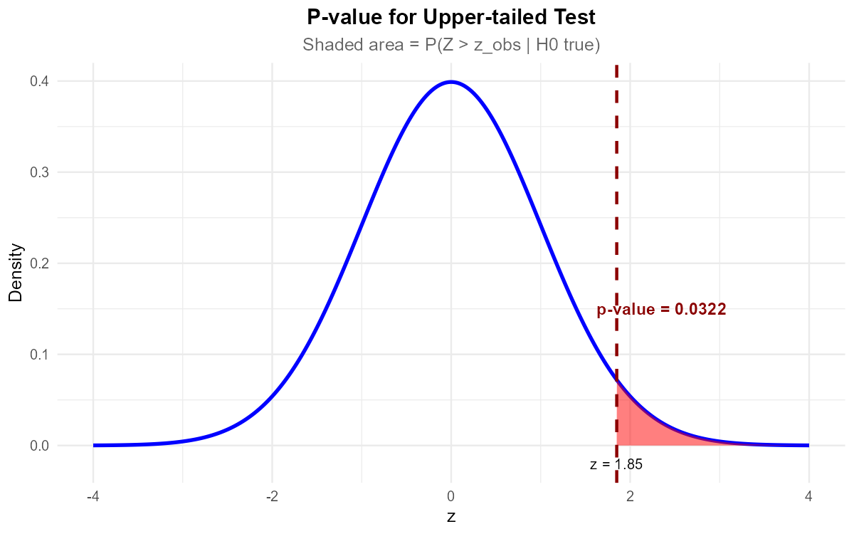
Fig. 10.19 P-value = shaded area in the tail beyond the observed test statistic.

\[p\text{-value} = P(Z > 1.60) = 0.0548\]

Part (d): Decision

Since p-value = 0.0548 > α = 0.05, fail to reject H₀.

Part (e): Interpretation

The data does not give support (p-value = 0.055) to the claim that the true mean response time exceeds 50 ms. The competitor cannot definitively disprove the company’s claim based on this sample.

R verification:

xbar <- 53.2; mu_0 <- 50; sigma <- 14; n <- 49
z_ts <- (xbar - mu_0) / (sigma / sqrt(n))  # 1.60
p_value <- pnorm(z_ts, lower.tail = FALSE)  # 0.0548

---

Exercise 4: P-value for Lower-tailed Test

A factory produces light bulbs with a historical mean lifetime of 1200 hours. After a process change, engineers suspect the lifetime may have decreased. They test n = 100 bulbs and find \(\bar{x} = 1175\) hours with σ = 120 hours (known from quality records).

1. State the hypotheses.

2. Calculate the z-test statistic.

3. Calculate the p-value.

4. At α = 0.05, what is the decision?

5. At α = 0.01, what is the decision?

Solution

Part (a): Hypotheses

Testing if lifetime has decreased:

\[H_0: \mu \geq 1200 \quad \text{vs} \quad H_a: \mu < 1200\]

Part (b): Z-test statistic

\[z_{TS} = \frac{1175 - 1200}{120 / \sqrt{100}} = \frac{-25}{12} = -2.083\]

Part (c): P-value (lower-tailed)

\[p\text{-value} = P(Z < -2.083) = 0.0186\]

Part (d): Decision at α = 0.05

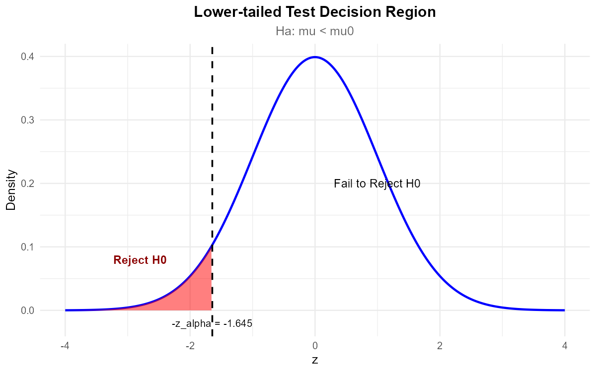
Fig. 10.20 Lower-tailed test: Reject H₀ when z_TS falls in the left tail.

Since p-value = 0.0186 < 0.05, reject H₀.

The data does give support (p-value = 0.019) to the claim that the mean bulb lifetime has decreased.

Part (e): Decision at α = 0.01

Since p-value = 0.0186 > 0.01, fail to reject H₀.

At the more stringent 1% level, the data does not give support to the claim.

R verification:

xbar <- 1175; mu_0 <- 1200; sigma <- 120; n <- 100
z_ts <- (xbar - mu_0) / (sigma / sqrt(n))  # -2.083
p_value <- pnorm(z_ts, lower.tail = TRUE)   # 0.0186

---

Exercise 5: P-value for Two-tailed Test

A manufacturing process targets mean weight of 500 g. Quality control samples n = 64 items and finds \(\bar{x} = 497.2\) g. Historical data shows σ = 15 g.

1. State the hypotheses (testing for any deviation from target).

2. Calculate the z-test statistic.

3. Calculate the p-value.

4. At α = 0.05, what is the decision?

5. At α = 0.10, what is the decision?

Solution

Part (a): Hypotheses

Testing if mean differs from target:

\[H_0: \mu = 500 \quad \text{vs} \quad H_a: \mu \neq 500\]

Part (b): Z-test statistic

\[z_{TS} = \frac{497.2 - 500}{15 / \sqrt{64}} = \frac{-2.8}{1.875} = -1.493\]

Part (c): P-value (two-tailed)

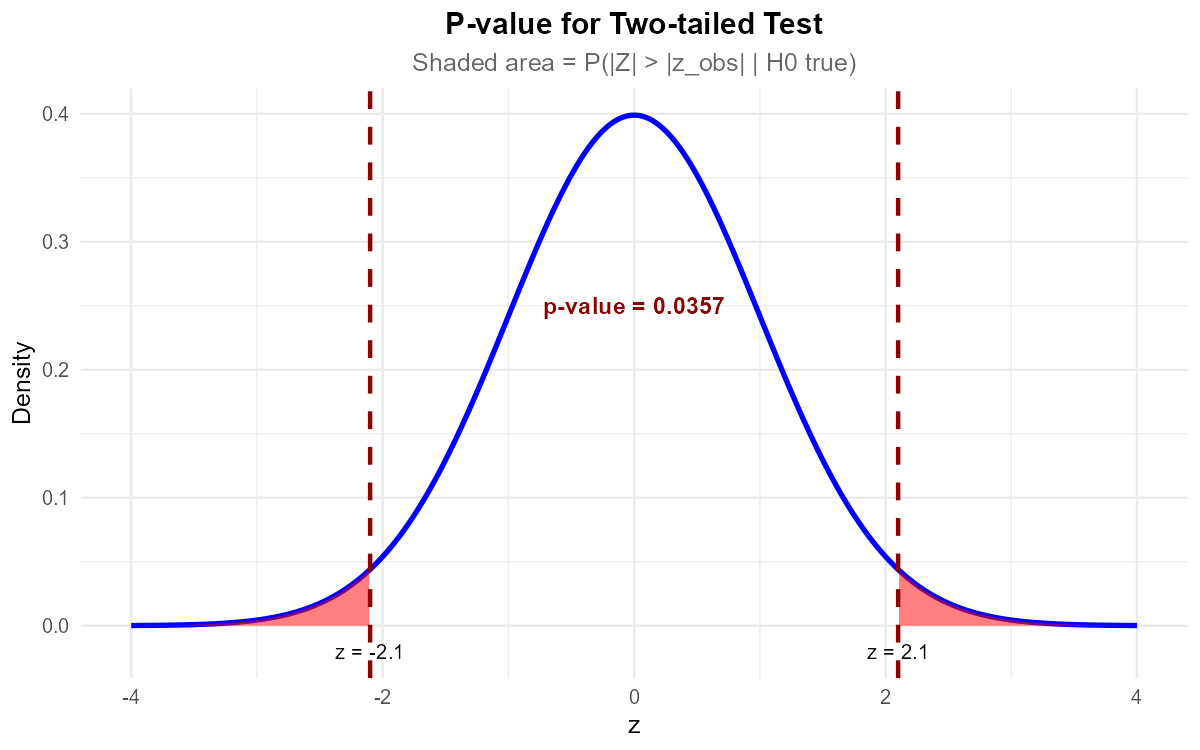
Fig. 10.21 For two-tailed tests, p-value includes both tails.

\[p\text{-value} = 2 \times P(Z > |{-1.493}|) = 2 \times P(Z > 1.493) = 2 \times 0.0677 = 0.1354\]

Part (d): Decision at α = 0.05

Since p-value = 0.1354 > 0.05, fail to reject H₀.

Part (e): Decision at α = 0.10

Since p-value = 0.1354 > 0.10, fail to reject H₀.

At both significance levels, the data does not give support to the claim that the mean differs from 500 g.

R verification:

xbar <- 497.2; mu_0 <- 500; sigma <- 15; n <- 64
z_ts <- (xbar - mu_0) / (sigma / sqrt(n))  # -1.493
p_value <- 2 * pnorm(abs(z_ts), lower.tail = FALSE)  # 0.1354

---

Exercise 6: Complete Z-Test (Upper-tailed)

A data center claims their servers maintain a mean CPU temperature of at most 70°C during peak load. An auditor wants to verify this claim. From extensive historical data, the population standard deviation is σ = 8°C. The auditor samples n = 40 measurements and finds \(\bar{x} = 72.5°C\). Use α = 0.05.

Perform a complete hypothesis test using the four-step framework.

Solution

Step 1: Define the Parameter

Let μ = true mean CPU temperature (°C) during peak load.

Step 2: State the Hypotheses

The auditor wants to show temperatures exceed the claimed maximum:

\[H_0: \mu \leq 70 \quad \text{vs} \quad H_a: \mu > 70\]

Step 3: Calculate Test Statistic and P-value

\[SE = \frac{\sigma}{\sqrt{n}} = \frac{8}{\sqrt{40}} = 1.265\]

\[z_{TS} = \frac{72.5 - 70}{1.265} = \frac{2.5}{1.265} = 1.977\]

P-value (upper-tailed):

\[p\text{-value} = P(Z > 1.977) = 0.0240\]

Step 4: Decision and Conclusion

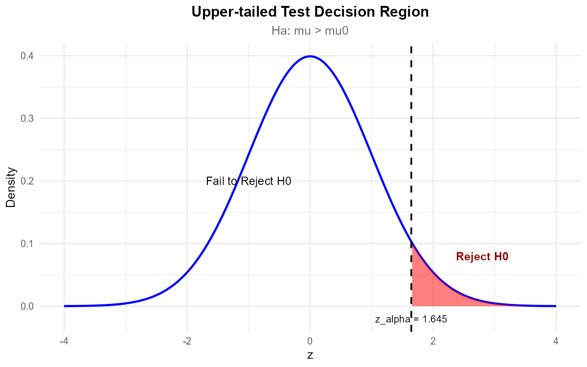
Fig. 10.22 Upper-tailed test: Reject H₀ when z_TS falls in the right tail.

Since p-value = 0.0240 < α = 0.05, reject H₀.

Conclusion: The data does give support (p-value = 0.024) to the claim that the true mean CPU temperature during peak load exceeds 70°C. The data center’s claim does not appear to be supported.

R verification:

xbar <- 72.5; mu_0 <- 70; sigma <- 8; n <- 40
SE <- sigma / sqrt(n)          # 1.265
z_ts <- (xbar - mu_0) / SE     # 1.977
p_value <- pnorm(z_ts, lower.tail = FALSE)  # 0.0240

---

Exercise 7: Complete Z-Test (Two-tailed)

A pharmaceutical company manufactures tablets with a target active ingredient of 250 mg. Regulatory standards require testing whether the mean differs from this target. Quality control tests n = 81 tablets and finds \(\bar{x} = 248.2\) mg. The population standard deviation is σ = 9 mg. Use α = 0.01.

Perform a complete hypothesis test using the four-step framework.

Solution

Step 1: Define the Parameter

Let μ = true mean active ingredient content (mg) per tablet.

Step 2: State the Hypotheses

Testing for any deviation from target:

\[H_0: \mu = 250 \quad \text{vs} \quad H_a: \mu \neq 250\]

Step 3: Calculate Test Statistic and P-value

\[SE = \frac{\sigma}{\sqrt{n}} = \frac{9}{\sqrt{81}} = 1.0\]

\[z_{TS} = \frac{248.2 - 250}{1.0} = -1.80\]

P-value (two-tailed):

\[p\text{-value} = 2 \times P(Z > |-1.80|) = 2 \times P(Z > 1.80) = 2 \times 0.0359 = 0.0719\]

Step 4: Decision and Conclusion

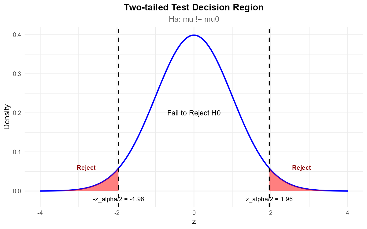
Fig. 10.23 Two-tailed test: Reject H₀ when |z_TS| falls in either tail.

Since p-value = 0.0719 > α = 0.01, fail to reject H₀.

Conclusion: The data does not give support (p-value = 0.072) to the claim that the mean active ingredient content differs from the target of 250 mg. The tablets appear to meet specifications.

R verification:

xbar <- 248.2; mu_0 <- 250; sigma <- 9; n <- 81
SE <- sigma / sqrt(n)          # 1.0
z_ts <- (xbar - mu_0) / SE     # -1.80
p_value <- 2 * pnorm(abs(z_ts), lower.tail = FALSE)  # 0.0719

---

Exercise 8: Decisions at Different Significance Levels

A researcher conducts a two-tailed z-test and obtains z_TS = 2.35.

1. Calculate the p-value.

2. At α = 0.10, what is the decision?

3. At α = 0.05, what is the decision?

4. At α = 0.01, what is the decision?

5. What is the smallest significance level at which H₀ would be rejected?

6. Explain why the decision can change depending on α.

Solution

Part (a): P-value

\[p\text{-value} = 2 \times P(Z > 2.35) = 2 \times 0.0094 = 0.0188\]

Part (b): Decision at α = 0.10

0.0188 < 0.10 → Reject H₀

Part (c): Decision at α = 0.05

0.0188 < 0.05 → Reject H₀

Part (d): Decision at α = 0.01

0.0188 > 0.01 → Fail to reject H₀

Part (e): Smallest α for rejection

The smallest α at which we would reject H₀ is the p-value itself: α = 0.0188

Any α ≥ 0.0188 leads to rejection; any α < 0.0188 leads to non-rejection.

Part (f): Why decisions vary with α

α represents our tolerance for Type I error. A smaller α means we require stronger evidence (smaller p-value) to reject H₀. The same data can lead to different conclusions depending on how stringent we set our criterion.

This highlights that statistical decisions involve a judgment call about acceptable error rates, not just mechanical calculation.

R verification:

z_ts <- 2.35
p_value <- 2 * pnorm(abs(z_ts), lower.tail = FALSE)  # 0.0188

---

Exercise 9: Application - Quality Assurance

An electronics manufacturer produces resistors with a nominal resistance of 1000 Ω. Historical process data shows σ = 25 Ω. Quality assurance tests a random sample of n = 50 resistors and measures \(\bar{x} = 1008.5\) Ω.

1. The QA engineer wants to test if the process mean differs from 1000 Ω at α = 0.05. Perform the complete hypothesis test.

2. Construct a 95% confidence interval for μ.

3. Verify that the CI and hypothesis test give consistent conclusions.

4. A customer requires that mean resistance be within ±5 Ω of 1000 Ω. Based on your analysis, does the process meet this specification?

Solution

Part (a): Hypothesis Test

Step 1: Let μ = true mean resistance (Ω).

Step 2: H₀: μ = 1000 vs Hₐ: μ ≠ 1000

Step 3:

\[SE = \frac{25}{\sqrt{50}} = 3.536\]

\[z_{TS} = \frac{1008.5 - 1000}{3.536} = 2.404\]

\[p\text{-value} = 2 \times P(Z > 2.404) = 0.0162\]

Step 4: Since 0.0162 < 0.05, reject H₀.

The data does give support (p-value = 0.016) to the claim that the mean resistance differs from 1000 Ω.

Part (b): 95% Confidence Interval

\[CI: \bar{x} \pm z_{0.025} \times SE = 1008.5 \pm 1.96 \times 3.536\]

\[= 1008.5 \pm 6.93 = (1001.57, 1015.43) \text{ Ω}\]

Part (c): Consistency Check

The null value μ₀ = 1000 is outside the 95% CI (1001.57, 1015.43).

By the duality principle, this means we should reject H₀ at α = 0.05, which matches our hypothesis test conclusion. ✓

Part (d): Customer Specification

The customer requires 995 ≤ μ ≤ 1005 Ω.

Our 95% CI is (1001.57, 1015.43), which extends beyond 1005 Ω.

The process does not appear to meet the customer’s specification. The mean resistance appears to be slightly high. Process adjustment may be needed to bring the mean closer to 1000 Ω.

R verification:

xbar <- 1008.5; mu_0 <- 1000; sigma <- 25; n <- 50
SE <- sigma / sqrt(n)  # 3.536
z_ts <- (xbar - mu_0) / SE  # 2.404
p_value <- 2 * pnorm(abs(z_ts), lower.tail = FALSE)  # 0.0162

# 95% CI
z_crit <- qnorm(0.025, lower.tail = FALSE)  # 1.96
c(xbar - z_crit * SE, xbar + z_crit * SE)  # (1001.57, 1015.43)

---

10.2.6. Additional Practice Problems

True/False Questions (1 point each)

1. A p-value of 0.03 means there’s a 3% probability that H₀ is true.

   Ⓣ or Ⓕ

2. If z_TS = 2.5 for an upper-tailed test, the p-value is P(Z > 2.5).

   Ⓣ or Ⓕ

3. For a test in the direction of the observed effect, the two-tailed p-value is twice the corresponding one-tailed p-value.

   Ⓣ or Ⓕ

4. If p-value = 0.04, we would reject H₀ at α = 0.05 but not at α = 0.01.

   Ⓣ or Ⓕ

5. The z-test requires that σ be known.

   Ⓣ or Ⓕ

6. A smaller p-value always indicates a larger effect size.

   Ⓣ or Ⓕ

Multiple Choice Questions (2 points each)

7. For a two-tailed z-test with z_TS = -1.96, the p-value is:

   Ⓐ 0.025

   Ⓑ 0.05

   Ⓒ 0.975

   Ⓓ 1.96

8. If \(\bar{x} = 42\), μ₀ = 40, σ = 10, n = 25, then z_TS equals:

   Ⓐ 0.2

   Ⓑ 1.0

   Ⓒ 2.0

   Ⓓ 5.0

9. The critical value for an upper-tailed test at α = 0.01 is:

   Ⓐ 1.645

   Ⓑ 1.96

   Ⓒ 2.326

   Ⓓ 2.576

10. A p-value of 0.07 leads to which decision at α = 0.05?

    Ⓐ Reject H₀

    Ⓑ Fail to reject H₀

    Ⓒ Accept H₀

    Ⓓ Cannot be determined

11. For a lower-tailed test with z_TS = -2.1, the p-value is:

    Ⓐ P(Z > 2.1)

    Ⓑ P(Z < -2.1)

    Ⓒ 2 × P(Z > 2.1)

    Ⓓ 1 - P(Z < -2.1)

12. Which provides the strongest evidence against H₀?

    Ⓐ p-value = 0.08

    Ⓑ p-value = 0.05

    Ⓒ p-value = 0.01

    Ⓓ p-value = 0.001

Answers to Practice Problems

True/False Answers:

1. False — The p-value is P(data as extreme | H₀ true), not P(H₀ true | data).

2. True — For upper-tailed tests, p-value = P(Z > z_TS).

3. True — When testing in the direction of the observed effect, the two-tailed p-value equals 2 × the one-tailed p-value.

4. True — 0.04 < 0.05 (reject), but 0.04 > 0.01 (fail to reject).

5. True — The z-test formula requires known σ; otherwise use t-test.

6. False — P-value also depends on sample size. Large n can produce small p-values even for tiny effects.

Multiple Choice Answers:

7. Ⓑ — Two-tailed: 2 × P(Z > 1.96) = 2 × 0.025 = 0.05.

8. Ⓑ — z_TS = (42 - 40)/(10/√25) = 2/2 = 1.0.

9. Ⓒ — z₀.₀₁ = 2.326 for upper-tailed at α = 0.01.

10. Ⓑ — 0.07 > 0.05, so fail to reject (never “accept”).

11. Ⓑ — Lower-tailed: p-value = P(Z < z_TS) = P(Z < -2.1).

12. Ⓓ — Smaller p-values indicate stronger evidence against H₀.