Slides 📊

• Hypothesis Testing for Single Sample (Part 1) (PPTX)

10.1. The Foundation of Hypothesis Testing

Hypothesis testing is a key statistical inference framework that assesses whether claims about population parameters are reasonable based on data evidence. In this lesson, we establish the basic language of hypothesis testing to prepare for the formal steps covered in the upcoming lessons.

Road Map 🧭

• Learn the building blocks of hypothesis testing.

• Formulate the null and alternative hypotheses in the correct format for a given research question.

• Understand the logic of constructing a decision rule.

• Recognize the two types of errors that can arise in hypothesis testing and understand how they are controlled or influenced by different components of the procedure.

10.1.1. The Building Blocks of Hypothesis Testing

A. The Dual Hypothesis Framework

A statistical hypothesis is a claim about one or more population parameters, expressed as a mathematical statement. The first step in hypothesis testing is to frame the research question as two competing hypotheses:

• Null hypothesis, \(H_0\): the status quo or a baseline claim, assumed true until there is sufficient evidence to conclude otherwise

• Alternative hypothesis, \(H_a\): the competing claim to be tested against the null

When testing a claim about the population mean \(\mu\), the hypothesis formulation follows a set of rules summarized by Fig. 10.1 and the following list.

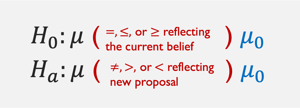
Fig. 10.1 Template for dual hypothesis

1. In Fig. 10.1, the part in black always stays unchanged.

2. \(\mu_0\), called the null value, is a point of comparison for \(\mu\) taken from the research context. It is represented with a symbol here, but it takes a concrete numerical value in applications.

3. \(H_0\) and \(H_a\) are complementary—their cases must not overlap yet together encompass all possibilities for the parameter. \(H_0\) always includes an equality sign (\(=, \leq, \geq\)), while the inequality in \(H_a\) is always strict (\(\neq, <, >\)).

Let us get some practice applying these rules correctly to research questions.

Example 💡: Writing the Hypotheses Correctly

For each research scenorio below, write the appropriate set of hypotheses to conduct a hypothesis test. Be sure to follow all the rules for hypotheses presentation.

1. The census data show that the mean household income in an area is $63K (63 thousand dollars) per year. A market research firm wants to find out whether the mean household income of the shoppers at a mall in this area is HIGHER THAN that of the general population.

   Let \(\mu\) denote the true mean household income of the shoppers at this mall. The dual hypothesis is:

   \[\begin{split}&H_0: \mu \leq 63\\ &H_a: \mu > 63\end{split}\]

   The question raised by the study will always align with the alternative hypothesis. Also note that the generalized symbol \(\mu_0\) in the template (Fig. 10.1) is replaced with a specific vlaue, 63, from the context.

2. Last year, your company’s service technicians took an average of 2.6 hours to respond to calls from customers. Do this year’s data show a DIFFERENT average time?

   Let \(\mu\) denote the true mean average response time by service techicians this year. The dual hypothesis appropriate for this research question is:

   \[\begin{split}&H_0: \mu = 2.6\\ &H_a: \mu \neq 2.6\end{split}\]

3. The drying time of paint under a specified test condition is known to be normally distributed with mean 75 min and standard deviation 9 min. Chemists have proposed a new additive designed to DECREASE average drying time. Should the company change to the new additive?

   Let \(\mu\) be the true mean drying time of the new paint formula. Then we have:

   \[\begin{split}&H_0: \mu \geq 75\\ &H_a: \mu < 75\end{split}\]

Three Types of Hypotheses

From these examples, we see that there are three main ways to formulate a pair of hypotheses. Focusing on the alternative side,

• A test with \(H_a: \mu > \mu_0\) is called an upper-tailed (right-tailed) hypothesis test.

• A test with \(H_a: \mu < \mu_0\) is called a lower-tailed (left-tailed) hypothesis test.

• A test with \(H_a: \mu \neq \mu_0\) is called a two-tailed hypothesis test.

B. The Significance Level

Before collecting any data, we must decide how strong the evidence must be to reject the null hypothesis. The significance level, denoted \(\alpha\), is the pre-specified probability that represents our tolerance for the error of rejecting a true null hypothesis. A small value, typically less than or equal to \(0.1\), is chosen based on expert recommendations, legal requirements, or field conventions. The smaller the \(\alpha\), the stronger the evidence must be to reject the null hypothesis.

C. The Test Statistic and the Decision

Identifying the Goal

For a concrete context, suppose we perform the upper-tailed hypothesis test for the true mean income of shoppers at a mall, taken from the first of the three examples above.

\[\begin{split}&H_0: \mu \leq 63\\ &H_a: \mu > 63\end{split}\]

Let us also assume that

1. \(X_1, X_2, \cdots, X_n\) form an iid sample from the population \(X\) with mean \(\mu\) and variance \(\sigma^2\).

2. Either the population \(X\) is normally distributed, or the sample size \(n\) is sufficiently large for the CLT to hold.

3. The population variance \(\sigma^2\) is known.

We now need to develop an objective rule for rejecting the null hypothesis. This rule must (1) be applicable in any upper-tailed hypothesis testing scenario where the assumptions hold, and (2) satisfy the maximum error tolerance condition given by \(\alpha\).

Finding the Decision Rule

It is natural to view the sample mean \(\bar{X}\) as central to the decision, since it is one of the best indicators of the true location of \(\mu\). In the simplest terms, if \(\bar{X}\) yields an observed value \(\bar{x}\) much larger than 63 (thousands of dollars), we would want to reject the null hypothesis, whereas if it is close to or lower than 63, there would not be enough evidence against it. The key question is, how large must \(\bar{x}\) be to count as sufficient evidence against the null?

Under the set of assumptions about the distribution of \(X\) and its sampling conditions, \(\bar{X}\) (approximately) follows a normal distribution. In addition, its full distribution can be given by

\[\bar{X} \sim N\left(63, \frac{\sigma^2}{n}\right)\]

under the null hypothesis. We call this the null distribution.

Let us consider rejecting the null hypothesis only if \(\bar{x}\) lands above the cutoff that marks an upper area of \(\alpha\) under the null distribution:

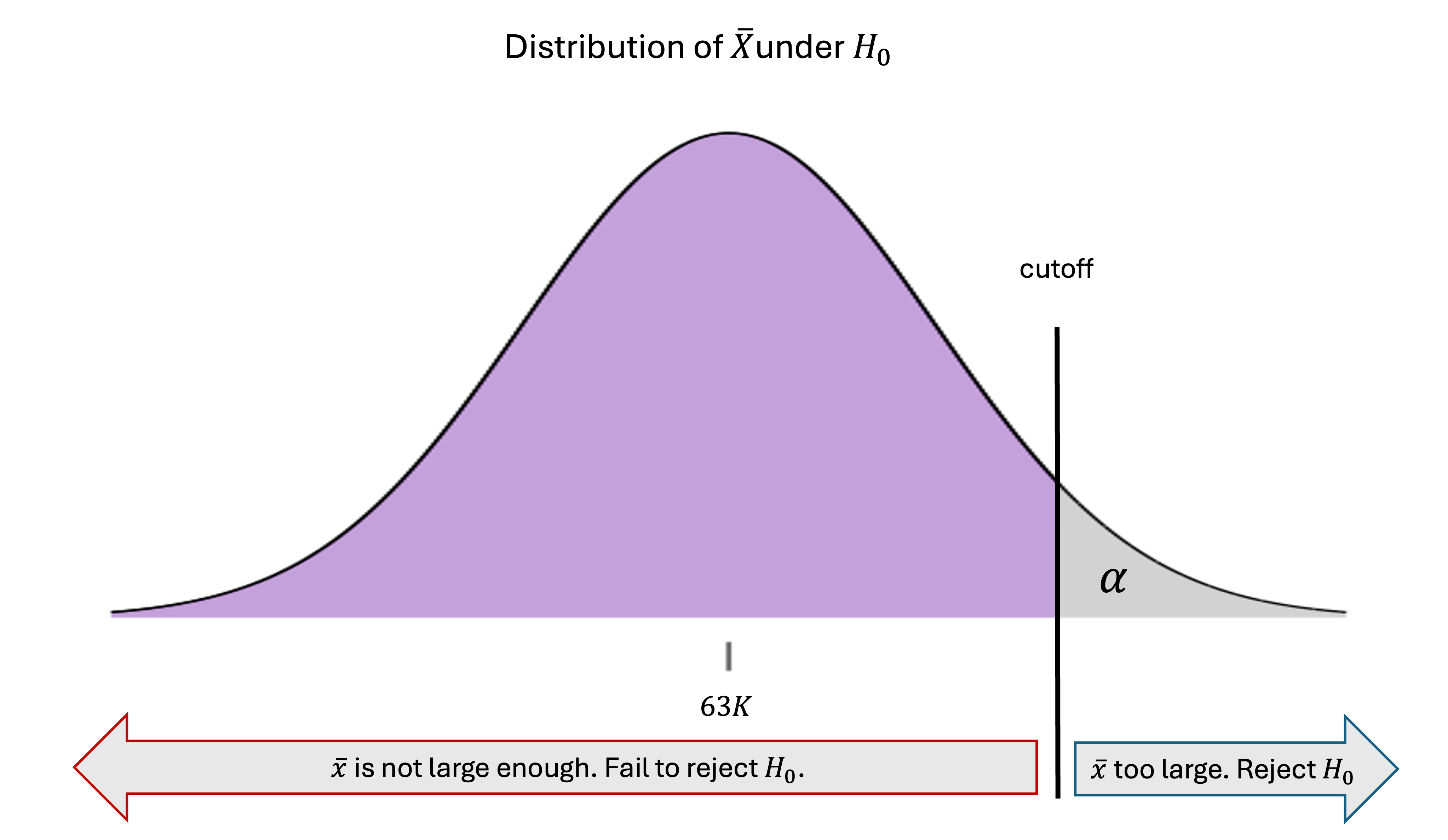
Fig. 10.2 Decision rule for an upper-tailed hypothesis test

1. Is this rule objective and universally applicable in other upper-tailed hypothesis tests?

   Yes. If the same set of assumptions hold, we can make an equivalent rule by replacing the values of \(\mu_0, \sigma^2\), and \(n\) appropriately.

2. Does this rule limit the false rejection rate to at most \(\alpha\) ?

   Yes. If \(H_0\) was indeed true, then according to the null distribution, \(\bar{X}\) would generate values above the cutoff only \(\alpha \cdot 100 \%\) of the time. By design, the chance of incorrectly rejecting the null hypothesis is limited by how often incorrect answers are generated under the null hypothesis.

3. What about other potential values under \(H_0\) ?

   The null hypothesis \(H_0: \mu \leq 63\) proposes that \(\mu\) is anything less than or equal to the null value, 63. Is the decision rule also safe for candidate values other than 63? The answer is yes. When the true mean is strictly less than \(\mu_0\), the entire distribution of \(\bar{X}\) slides to the left and away from the cutoff, leaving an upper-tail area smaller than \(\alpha\):

   

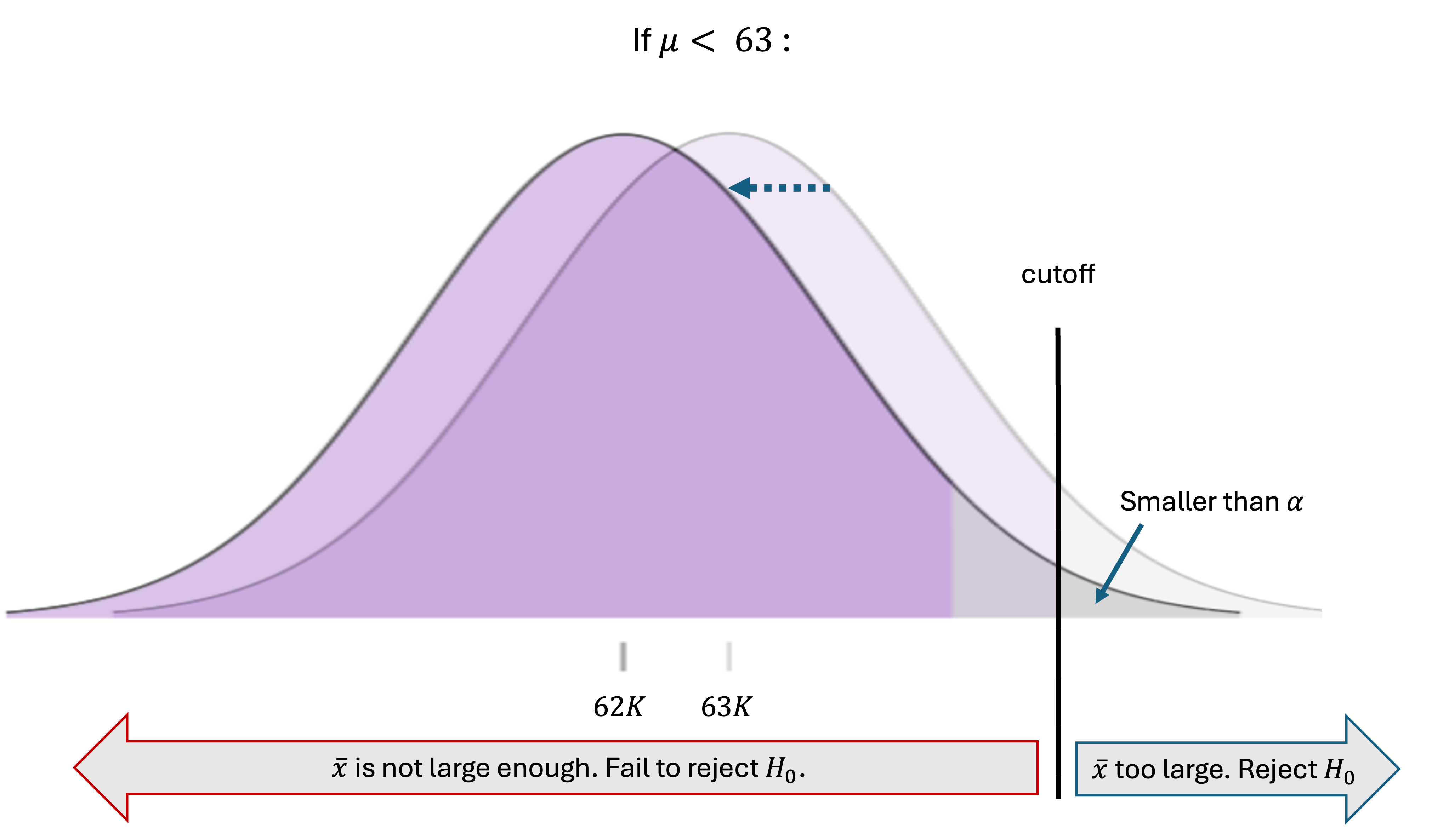
   Fig. 10.3 Candicate values for \(\mu\) other than \(\mu_0\) in the null hypothesis

   Therefore, error-inducing outcomes are generated even less frequently than when the population mean is exactly 63. In general, the boundary case of \(\mu=\mu_0\) addresses the worst case scenario in terms of false rejection rates. If the rule is safe under the boundary case, then it is safe under all other scenarios belonging to the null hypothesis.

How to Locate the Cutoff

The exact location of the cutoff can be computed by viewing it as a \((1-\alpha)\cdot 100\)-th percentile of the boundary case null distribution. Using the techniques learned in Chapter 6, confirm that the cutoff is \(z_{\alpha}\frac{\sigma}{\sqrt{n}} + 63\) for this example, where \(z_\alpha\) is the \(z\)-critical value used in Chapter 9. In general,

\[\text{cutoff}_{upper} = z_{\alpha}\frac{\sigma}{\sqrt{n}} + \mu_0.\]

In summary, we reject the null hypothesis of an upper-tailed hypothesis test if \(\bar{x} > z_{\alpha}\frac{\sigma}{\sqrt{n}} + \mu_0\) or, by standardizing both sides, if

\[\frac{\bar{x}-\mu_0}{\sigma/\sqrt{n}} > z_{\alpha}.\]

What About the Cutoff for a Lower-Tailed Hypothesis Test?

By making a mirror argument of this section, confirm that you would reject the null hypothesis for a lower-tailed hypothesis test if \(\bar{x} < -z_\alpha\frac{\sigma}{\sqrt{n}} + \mu_0 = \text{cutoff}_{lower}\), or by standardizing both sides, if

\[\frac{\bar{x}-\mu_0}{\sigma/\sqrt{n}} < -z_{\alpha}.\]

The Test Statistic

A statistic that measures the consistency of the observed data with the null hypothesis is called the test statistic. For hypothesis tests on a population mean, \(\frac{\bar{X}-\mu_0}{\sigma/\sqrt{n}}\) plays this role. Its realized value represents the standardized distance between the hypothesized true mean \(\mu_0\) and the generated outcome \(\bar{x}\). It is also used for comparison against a \(z\)-critical value to draw the final decision. Since it follows the standard normal distribution under the null hypothesis, we denote this quantity \(Z_{TS}\):

\[Z_{TS} = \frac{\bar{X}-\mu_0}{\sigma/\sqrt{n}}\]

and call it the \(z\)-test statistic.

10.1.2. Understanding Type I and Type II Errors

Since the results of hypothesis tests always accompany a degree of uncertainty, it is important to analyze the likelihood and consequences of the possible errors. There are two types of errors that can arise in hypothesis testing. The error of incorrectly rejecting a true null hypothesis is called the Type I error, while the error of failing to reject a false null hypothesis is called the Type II error. The table below summarizes the different combinations of reality and decision.

Decision		Fail to Reject \(H_0\)	Reject \(H_0\)
Reality	\(H_0\) is True	✅ Correct	❌ Type I Error
	\(H_0\) is False	❌ Type II Error	✅ Correct

Type I Error: False Positive

A Type I error occurs when a true null hypothesis is rejected. This error results in a false positive claim of an effect or difference when none actually exists. The probability of making a Type I error is denoted \(\alpha\). Formally,

\[\alpha = P(\text{Type I error}) = P(\text{Reject } H_0|H_0 \text{ is true}).\]

Examples of Type I errors

• Concluding that a new drug is effective when it actually has no effect

• Claiming that a manufacturing process has changed when it is operating the same way as before

Type II Error: False Negative

A Type II error occurs when a false null hypothesis is not rejected. This results in a false negative case where real effect or difference goes undetected. The probability of making a Type II error is

\[\beta = P(\text{Type II error}) = P(\text{Fail to reject } H_0| H_0 \text{ is false}).\]

Examples of Type II errors

• Failing to detect that a new drug is more effective than placebo

• Failing to recognize that a manufacturing process has deteriorated

Error Trade-offs and Prioritization of the Type I Error

Type I and Type II errors are inversely related—efforts to reduce one type of error typically increase the other. The only way to reduce both error types simultaneously is to increase the sample size, collect higher quality data, or improve the measurement process.

When constructing a hypothesis test under limited resources, therefore, we must prioritize one error over the other. We typically choose to control \(\alpha\). That is, we design the decision-making procedure so that its probability of Type I error reamins below a pre-specified maximum. We make this choice because falsely claiming change from the status quo often carries substantial immediate cost. Such costs can include purchasing new factory equipment, setting up a production line and marketing strategy for a new drug, or revising a business contract.

By consequence, we cannot directly control \(\beta\). Instead, we analyze and try to minimize \(\beta\) by learning its relationship with the population distribution, sample size, and the significance level \(\alpha\).

A Legal System Analogy 🧑‍⚖️

The analogy between hypothesis testing and the American legal system offers useful insight. Just as we would rather let a guilty person go free than convict an innocent person, we are generally more concerned about incorrectly rejecting a true null hypothesis than about failing to detect a false one. Further,

• The null hypothesis is like the defendant, presumed innocent until proven guilty.

• The alternative hypothesis is like the prosecutor, trying to establish the defendant’s guilt.

• The significance level \(\alpha\) represents the standard of evidence required for conviction.

• The test statistic summarizes all the evidence presented at trial.

• The p-value (to be discussed in Section 10.2) measures how convincing this evidence is.

10.1.3. Statistical Power: The Ability to Detect True Change

Definition

Statistical power is the probability that a test will correctly reject a false null hypothesis. It represents the test’s ability to detect an unusual effect when it actually exists. It is also the complement of the Type II error probability, \(\beta\).

\[\text{Power} = P(\text{Reject } H_0 | H_0 \text{ is false}) = 1 - \beta\]

Power ranges from 0 to 1, with higher values indicating a better ability to detect false null hypotheses. A power of 0.80 means that if the null hypothesis is false, the test correctly rejects it with 80% chance.

Visualization of \(\alpha, \beta\), and Power

Let us continue with the upper-tailed hypothesis test for the true mean household income of shoppers at a mall. The dual hypothesis is:

\[\begin{split}&H_0: \mu \leq 63\\ &H_a: \mu > 63\end{split}\]

where the null value is \(\mu_0 = 63\). We agreed to reject the null hypothesis whenever \(\bar{x}\) was “too large”, or when

\[\bar{x} > z_{\alpha}\frac{\sigma}{\sqrt{n}} + 63 = \text{cutoff}_{upper}.\]

Let us also make the unrealistic assumption that we know the true value of \(\mu\); it is equal to \(\mu_a = 65,\) making the reality belong to the alternative side. Let us visualize this along with the resulting locations of \(\alpha\), \(\beta\), and power:

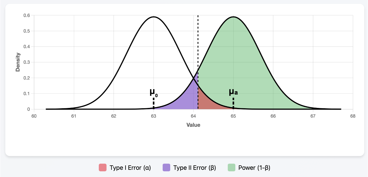
Fig. 10.4 Plots were generated using \(n=35, \mu_0 = 63, \mu_a=65, \sigma=4, \alpha =0.05\) in 🔗 Power Simulator .

The diagram has two normal densities partially overlapping one another. The left curve, centered at \(\mu_0 = 63\), represents the reality assumed by the null hypothesis, while the right curve, centered at \(\mu_a=65,\) represents the truth. According to our decision rule, we draw the cutoff where it leaves an upper-tail area of \(\alpha\) (red) under the null distribution and reject the null hypothesis whenever we see the sample mean land above it.

What happens if, in the meantime, the sample means are actually being generated from the right (alternative) curve? With probabiliy \(\beta\) (purple), it will generate an observed sample mean that will fail to lead to a rejection of \(H_0\) (Type II error). All other outcomes will lead to a correct rejection, with the probability represented by the green area (power).

Let us observe how the sizes of these three regions are influenced by different components of the experiment.

What Influcences Power?

Significance Level, \(\alpha\)

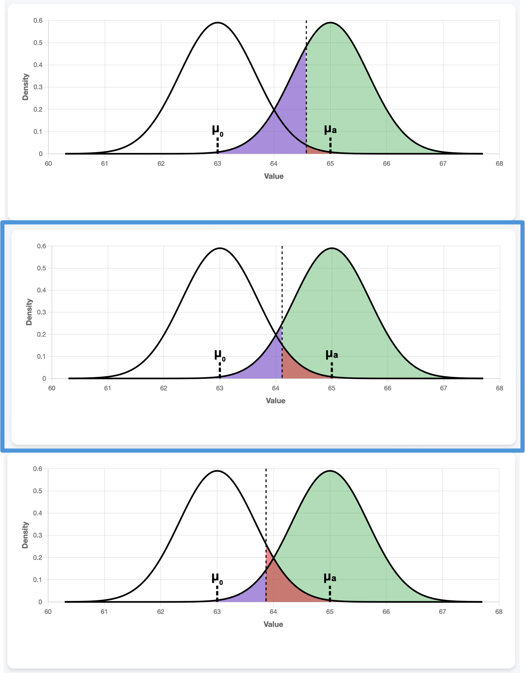
Fig. 10.5 \(\alpha=0.01, 0.05, 0.1\) from top to bottom

The central plot with the blue outline is the original plot, identical to Fig. 10.4. A smaller \(\alpha\) pushes the cutoff up in an upper-tailed hypothesis test, since it calls for more caution against Type I error and requires a stronger evidence (larger \(\bar{x}\)) for rejection of the null hypothesis. In response, the probability of Type II error increases (purple) and the power decreases (green).

True Mean, \(\mu_a\)

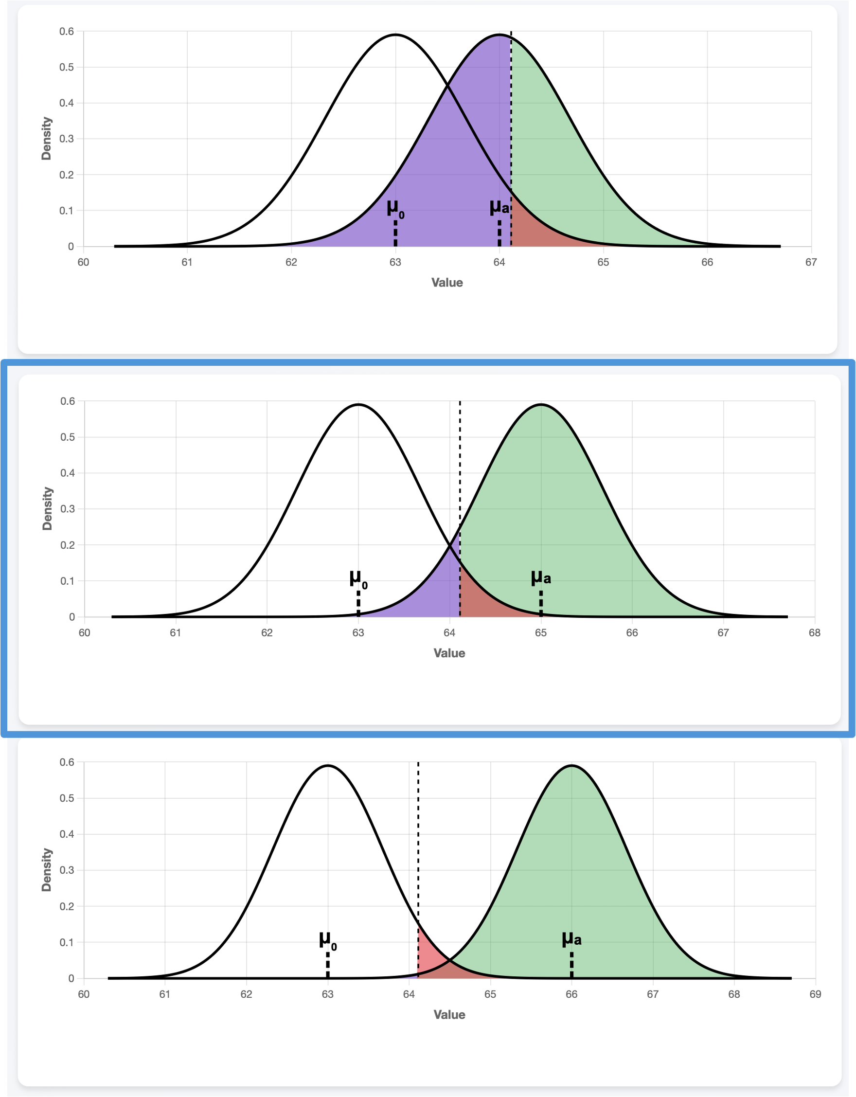
Fig. 10.6 \(\mu_a=64,65,66\) from top to bottom

If the hypothesized \(\mu_0\) and the true effect \(\mu_a\) are close to each other, it is naturally harder to separate the two cases. Even though \(\alpha\) stays constant (because we explicitly control it), the power decreases and the Type II error probability goes up as the distance between \(\mu_0\) and \(\mu_a\) narrows.

Population Standard Deviation, \(\sigma\)

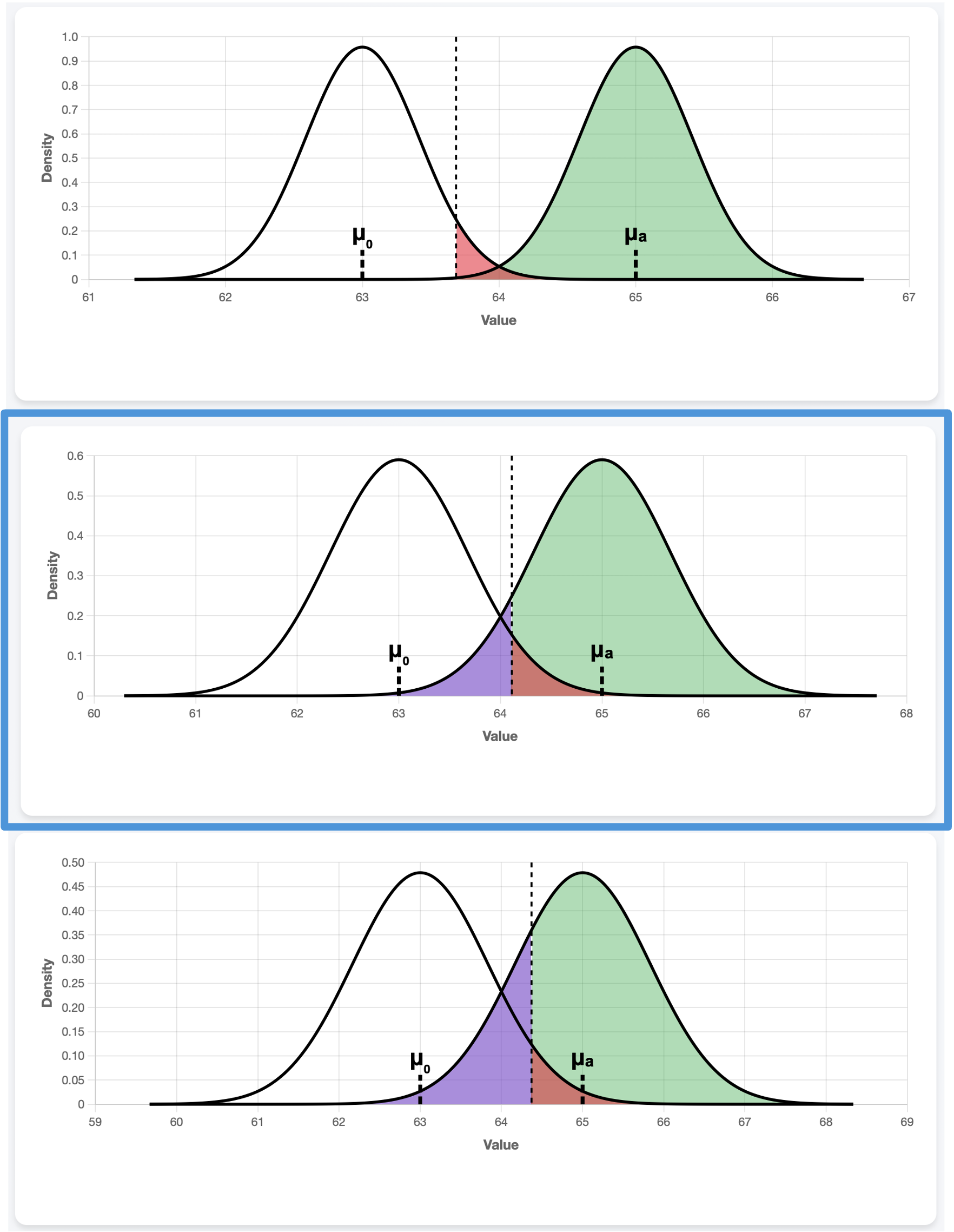
Fig. 10.7 \(\sigma=2.5, 4, 5\) from top to bottom

Recall that \(\bar{X}\) has the standard deviation \(\sigma/\sqrt{n}\). When \(\sigma\) decreases while \(\mu_0\) and \(\mu_a\) stay constant, the two densities become narrower around their respective means, creating a stronger separation between the two cases. This leads to a higher power and smaller Type II error probability.

Sample Size, \(n\)

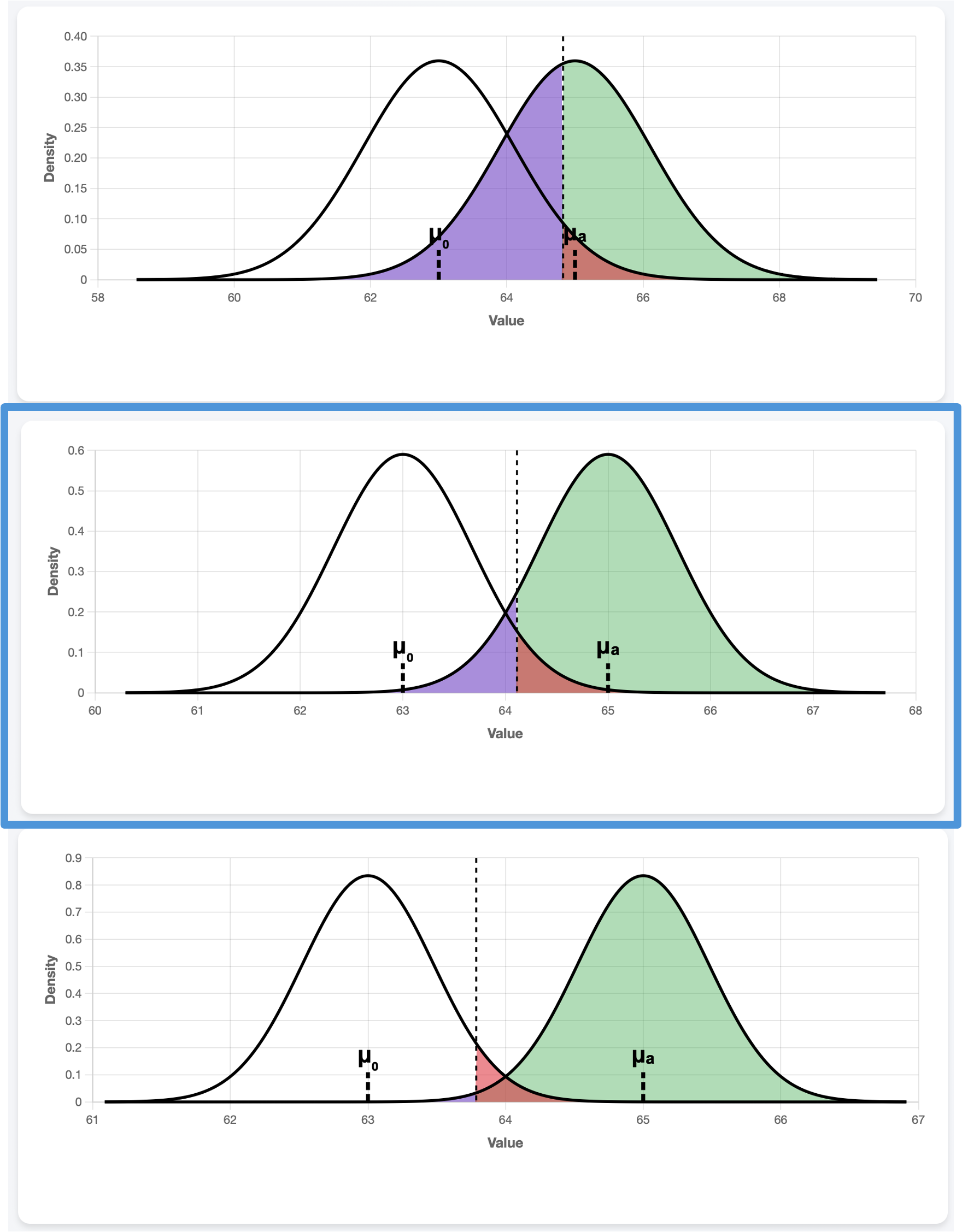
Fig. 10.8 \(n=13, 35, 70\) from top to bottom

The sample size \(n\) also affects the spread of the distribution of \(\bar{X}\), but in the opposite direction of \(\sigma\). As \(n\) decreases, \(\sigma/\sqrt{n}\) increases, making the densities wider. Larger overlap between the distributions leads to decreased power and higher Type II error probability.

Power Analysis Simulator 🎮

Explore how \(\alpha, \beta\), and statistical power relate to each other, and reproduce the images used in this section using:

🔗 Interactive Demo | 📄 R Code

10.1.4. Prospective Power Analysis

From the previous discussion, we find that the only realistic way to control statistical power is through the sample size, \(n\). Before conducting a study, researchers perform prospective power analysis to determine the sample size needed to ensure adequate power in their tests.

We continue with the upper-tailed hypothesis test on the true mean household income of shoppers at a mall:

\[\begin{split}&H_0: \mu \leq 63\\ &H_a: \mu > 63\end{split}\]

Suppose that the researchers expect the test to detect an increase of 2K in the household income effectively. Specifically, such jump should be detected with a probability at least 0.8. In other words, we want:

\[\text{Power} = 1-\beta \geq 0.8\]

when \(\mu = 63 + 2 = 65\). The magnitude of change to be detected, 2 in this case, is also called the effect size.

Additionally, we still assume:

1. \(X_1, X_2, \cdots, X_n\) forms an iid sample from a population \(X\) with mean \(\mu\) and variance \(\sigma^2\).

2. Either the population \(X\) is normally distributed, or the sample size \(n\) is sufficiently large for the CLT to hold.

3. The population variance \(\sigma^2\) is known.

Step 1: Mathematically Clarify the Goal

In general, \(\text{Power} = P(\text{Reject} H_0|H_0 \text{ is false})\).

We replace the general definition with the specific conditions given by our problem. The event of “rejecting \(H_0\)” is equivalent to the event \(\{\bar{X} > \text{cutoff}_{upper}\},\) and the event that \(H_0\) is false should now reflect the desired effect size. Therefore, our goal is to find \(n\) satisfying:

\[\text{Power} = P\left(\bar{X} > \text{cutoff}_{upper} \Bigg| \mu=65\right) \geq 0.8\]

or, equivalently,

\[\beta = P\left(\bar{X} \leq \text{cutoff}_{upper} \Bigg| \mu=65\right) < 0.2.\]

Denote the value \(0.2\) by \(\beta_{max}\), since we do not allow \(\beta\) to be larger than \(0.2\).

Step 2: Simplify and Calculate

Let us break down the latter form of our mathematical goal.

• From the conditional information, we know that \(\bar{X}\) is assumed to follow the distribution \(N(65, \sigma/\sqrt{n})\).

• Since the goal is written with a strict inequality, the cutoff must be a value strictly less than the 20th (\(\beta_{max}\cdot 100\)-th) percentile of \(N(65, \sigma/\sqrt{n})\). Mathematically,

  \[\text{cutoff}_{upper} < -z_{\beta_{max}}\frac{\sigma}{\sqrt{n}} + 65\]

  where \(z_{\beta_{max}}\) is a \(z\)-critical value computed for the upper-tail area \(\beta_{max}\).

• Replacing the \(\text{cutoff}_{upper}\) with its complete formula,

  \[z_\alpha\frac{\sigma}{\sqrt{n}} + 63 < -z_{\beta_{max}}\frac{\sigma}{\sqrt{n}} + 65.\]

  Isolate \(n\):

  \[n > \left(\frac{(z_{\alpha} + z_{\beta_{max}}) \sigma}{65 - 63}\right)^2.\]

Since \(n\) must be an integer, we take the smallest integer above this lower bound.

Summary

In an upper-tailed hypothesis test, the minimum sample size for a desired power lower bound \(1-\beta_{max}\) and an effect size \(|\mu_a-\mu_0|\) is the smallest integer \(n\) satisfying:

\[n > \left(\frac{(z_{\alpha} + z_{\beta_{\max}}) \sigma}{|\mu_a - \mu_0|}\right)^2.\]

Prospective Power Analysis for Lower-tailed Hypothesis Tests

By walking through a mirror argument, confirm that the minimum sample size \(n\) for a desired power lower bound \(1-\beta_{max}\) and an effect size \(|\mu_a-\mu_0|\) in a lower-tailed hypothesis test is determined by the same formula as the upper-tailed case.

Example 💡: Compute Power for SAT Scores

A teacher at STAT High School believes that their students score higher on the SAT than the 2013 national average of 1497. Assume the true standard deviation of SAT scores from this school is 200.

Q1: The teacher wants to construct a hypothesis test at 0.01 significance level that can detect a 20-point increase in the true mean effectively. If the current sample size is 300, what is the power of this test?

Step 1: Identify the Components

• The dual hypothesis is:

  \[\begin{split}&H_0: \mu \leq 1497\\ &H_a: \mu > 1497\end{split}\]

• \(\alpha = 0.01\) (\(z_{0.01} = 2.326348\))

  z_alpha <- qnorm(0.01, lower.tail = FALSE)
  

• Effect size: \(20\) points. This makes \(\mu_a = \mu_0 + 20 = 1497 = 1517\).

• Population standard deviation is \(\sigma = 200\) points

• Current sample size: \(n=300\)

Step 2: Find the Cutoff

\[\text{cutoff}_{upper} = 1497 + \frac{200}{\sqrt{300}}(2.326348) = 1497 + 26.862 = 1523.862\]

Step 3: Calculate Power

\[\text{Power} = P(\bar{X} > 1523.862 | \mu = 1517)\]

Using the conditional information, we compute the probability assuming that \(\bar{X} \sim N(1517, \sigma/\sqrt{n})\).

\[\begin{split}\text{Power} &= P\left(\frac{\bar{X}-1517}{\sigma/\sqrt{n}} > \frac{1523.862-1517}{\sigma/\sqrt{n}}\right)\\ &= P(Z > 0.5943) = 0.2762\end{split}\]

Result: The power is only 27.62%. This test is not sufficiently sensitive to reliably detect a 20-point improvement.

Example 💡: Compute Minimum Sample Size for SAT Scores

Q2: Continuing with the SAT scores problem, what is the minimum sample size required for the test to detect a 20-point increase with at least 90% chance?

Step 1: Identify the Components

• \(\text{Power} \geq 0.90\) is required, so \(\beta = 1 - \text{Power} < 0.10 = \beta_{max}\).

• \(z_{\beta_{max}} = 1.282\)

  z_betamax <- qnorm(0.1, lower.tail=FALSE)
  

Step 2: Apply the Formula

\[\begin{split}n &> \left[\frac{(z_{\alpha} + z_{\beta_{max}}) \sigma}{|\mu_a - \mu_0|}\right]^2 = \left[\frac{(2.326348 + 1.281552)(200)}{1517-1497}\right]^2\\ &= \left[\frac{(3.6079)(200)}{20}\right]^2 = (36.079)^2 = 1301.69\end{split}\]

Result: We would need at least \(n = 1302\) students to achieve 90% power—much larger than the available sample of 300.

Example 💡: Average Recovery Time

A pharmaceutical company wants to test whether a new drug reduces average recovery time from a common illness. Historical data shows the standard recovery time is \(\mu_0 = 7\) days with \(\sigma = 2\) days. The company wants to detect a reduction to \(\mu_a = 6\) days (a 1-day improvement) with 90% power at \(\alpha = 0.05\) significance.

Step 1: Identify the Components

• The hypotheses

  \[\begin{split}&H_0: \mu \geq 7\\ &H_a: \mu < 7\end{split}\]

• The significance level: \(\alpha = 0.05\) \((z_{\alpha} = 1.645)\)

  z_alpha <- qnorm(0.05, lower.tail=FALSE)
  

• \(\text{Power} \geq 0.90\) is required, so \(\beta = 1 - \text{Power} < 0.10 = \beta_{max}\). \((z_{\beta_{max}} = 1.282)\)

  z_betamax <- qnorm(0.1, lower.tail=FALSE)
  

• Effect size: \(|\mu_a - \mu_0| = |6 - 7| = 1\) day

• Population standard deviation: \(\sigma = 2\) days

Step 2: Calculate Required Sample Size

\[\begin{split}n &> \left(\frac{(1.645 + 1.282)(2)}{|6 - 7|}\right)^2 \\ &= \left(\frac{(2.927)(2)}{1}\right)^2 = (5.854)^2 \approx 34.3\end{split}\]

The company needs at least \(n = 35\) patients to achieve statistical power of at least 90%.

10.1.5. Bringing It All Together

Key Takeaways 📝

1. Hypothesis testing provides a framework for evaluating specific claims about population parameters using sample evidence. It consists of formally presenting the null and alternative hypotheses, determining the significance level, computing a test statistic, determining its strength, and drawing a decision.

2. Type I error (false positive) occurs when a true null hypothesis is rejected. Its probability, denoted \(\alpha\), is the significance level of the test.

3. Type II error (false negative) occurs whe a false null hypothesis is not rejected. It occurs with probability \(\beta\).

4. Statistical power (1-\(\beta\)) measures a test’s ability to detect false null hypotheses. It depends on the sample size, significance level, and population standard deviation.

10.1.6. Exercises

Exercise 1: Writing Hypotheses Correctly

For each research scenario, write the appropriate null and alternative hypotheses. Define the parameter of interest and identify whether the test is upper-tailed, lower-tailed, or two-tailed.

1. A pharmaceutical company claims their new drug reduces average recovery time from 7 days. Researchers want to test this claim.

2. A quality engineer suspects that a manufacturing process is producing bolts with mean diameter different from the target of 10 mm.

3. An environmental agency wants to verify that mean pollution levels do not exceed the safety threshold of 50 ppm.

4. A software company claims their new algorithm reduces average processing time below the industry standard of 200 ms.

5. A nutritionist wants to test whether a new diet changes average weight loss from the typical 5 pounds per month.

Solution

Part (a): Drug recovery time

Let μ = true mean recovery time (days) with the new drug.

\[H_0: \mu \geq 7 \quad \text{vs} \quad H_a: \mu < 7\]

Lower-tailed test (testing if recovery time is less than 7 days)

Part (b): Bolt diameter

Let μ = true mean bolt diameter (mm).

\[H_0: \mu = 10 \quad \text{vs} \quad H_a: \mu \neq 10\]

Two-tailed test (testing if diameter is different from target)

Part (c): Pollution levels

Let μ = true mean pollution level (ppm).

\[H_0: \mu \leq 50 \quad \text{vs} \quad H_a: \mu > 50\]

Upper-tailed test (testing if pollution exceeds threshold)

Note: This is the standard regulatory framing—we protect against exceeding the threshold by placing it in H₀. Rejecting H₀ triggers action.

Part (d): Processing time

Let μ = true mean processing time (ms) with new algorithm.

\[H_0: \mu \geq 200 \quad \text{vs} \quad H_a: \mu < 200\]

Lower-tailed test (testing if time is less than standard)

Part (e): Weight loss

Let μ = true mean monthly weight loss (pounds) with new diet.

\[H_0: \mu = 5 \quad \text{vs} \quad H_a: \mu \neq 5\]

Two-tailed test (testing if weight loss is different from typical)

---

Exercise 2: Identifying Type I and Type II Errors

For each scenario, describe in context what constitutes a Type I error and a Type II error.

1. Testing whether a new battery lasts longer than 20 hours on average.

   • \(H_0: \mu \leq 20\) vs \(H_a: \mu > 20\)

2. Testing whether a medical diagnostic test correctly identifies a disease (null: patient is healthy).

   • \(H_0:\) Patient is healthy vs \(H_a:\) Patient has disease

3. Testing whether a defendant is guilty in a criminal trial.

   • \(H_0:\) Defendant is innocent vs \(H_a:\) Defendant is guilty

4. For each scenario above, which error would you consider more serious? Explain.

Solution

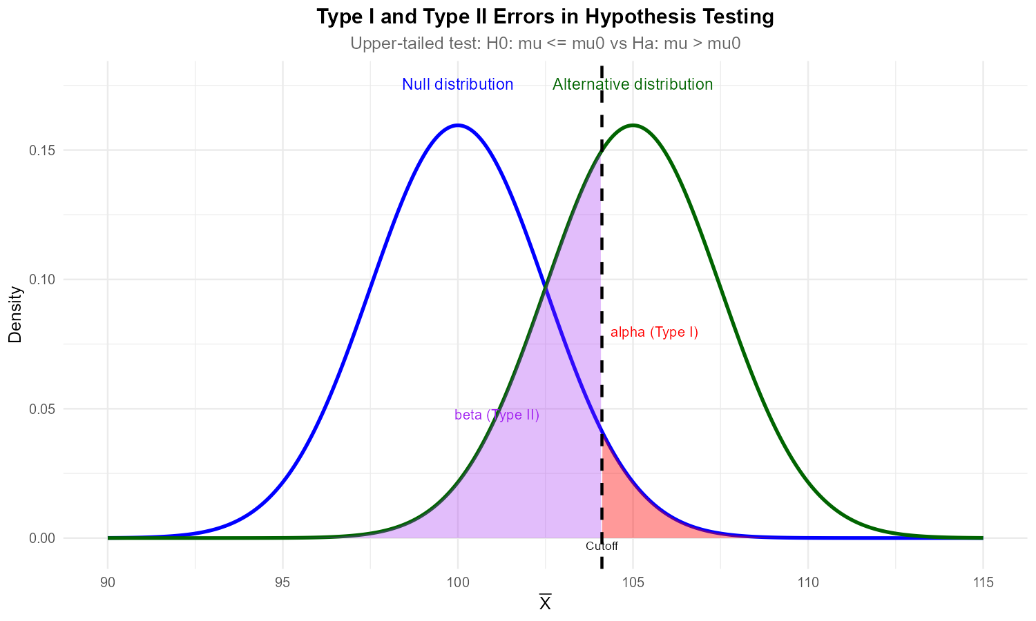
Fig. 10.9 Type I error (α): Rejecting H₀ when true. Type II error (β): Failing to reject H₀ when false.

Part (a): Battery life test

• Type I Error: Conclude the battery lasts longer than 20 hours when it actually doesn’t. The company might market an inferior product based on false claims.

• Type II Error: Fail to detect that the battery lasts longer than 20 hours when it actually does. The company might miss an opportunity to market a superior product.

Part (b): Medical diagnostic test

• Type I Error: Diagnose disease when patient is healthy (false positive). Patient undergoes unnecessary treatment, experiences anxiety, and incurs costs.

• Type II Error: Fail to detect disease when patient is sick (false negative). Patient doesn’t receive needed treatment, potentially leading to worse outcomes.

Part (c): Criminal trial

• Type I Error: Convict an innocent person. An innocent person loses freedom and suffers unjust punishment.

• Type II Error: Acquit a guilty person. A criminal goes free and may commit more crimes.

Part (d): Which error is more serious?

Note: The relative seriousness depends on context—costs, consequences, and stakeholders vary by situation.

• Battery: Type I error is more serious—it could lead to customer dissatisfaction, warranty costs, and damage to company reputation.

• Medical test: Type II error is often more serious—missing a disease can be life-threatening. However, this depends on the disease severity and treatment side effects.

• Criminal trial: Type I error is generally considered more serious—“better that ten guilty persons escape than that one innocent suffer” (Blackstone’s ratio). Our justice system is designed to minimize convicting innocents (α is very small).

---

Exercise 3: Understanding Significance Level

1. Define the significance level (α) in your own words.

2. A researcher sets α = 0.05. Interpret what this means in the context of hypothesis testing.

3. If a researcher uses α = 0.01 instead of α = 0.05, how does this affect:

   1. The probability of Type I error?

   2. The probability of Type II error?

   3. The power of the test?

4. Why don’t researchers always use a very small α (like 0.001)?

Solution

Part (a): Definition

The significance level (α) is the maximum probability of committing a Type I error that the researcher is willing to tolerate. It represents our tolerance for incorrectly rejecting a true null hypothesis.

Part (b): Interpretation of α = 0.05

The researcher accepts a 5% chance of rejecting H₀ when H₀ is actually true. If the test is repeated many times under conditions where H₀ is true, about 5% of the tests would incorrectly reject H₀.

Part (c): Effects of reducing α from 0.05 to 0.01

(i) Probability of Type I error decreases from 0.05 to 0.01.

(ii) Probability of Type II error increases. Making it harder to reject H₀ means we’re more likely to fail to reject a false H₀.

(iii) Power decreases. Since Power = 1 - β and β increases, power decreases.

Part (d): Why not always use very small α?

• Tradeoff with Type II error: Very small α dramatically increases β, making it very hard to detect real effects.

• Sample size requirements: Achieving reasonable power with small α requires much larger samples.

• Practical significance: An extremely stringent α may be unnecessary for many applications.

• Cost-benefit: The cost of Type I vs Type II errors should guide α selection, not a desire for extreme caution.

---

Exercise 4: Error Probability Calculations

A quality control test has α = 0.05. The test has 80% power to detect when the process mean shifts from 100 to 105.

1. What is the probability of a Type I error?

2. What is the probability of a Type II error (when μ = 105)?

3. If we test 100 batches where the true mean is actually 100, how many would we expect to incorrectly reject?

4. If we test 100 batches where the true mean has shifted to 105, how many would we expect to correctly detect this shift?

Solution

Part (a): Type I error probability

P(Type I Error) = α = 0.05

Part (b): Type II error probability

Power = 1 - β = 0.80, so β = 1 - 0.80 = 0.20

Part (c): False rejections out of 100 (H₀ true)

Expected = n × α = 100 × 0.05 = 5 batches

These would be false alarms—incorrectly flagging batches as having shifted when they haven’t.

Part (d): Correct detections out of 100 (H₀ false, μ = 105)

Expected = n × Power = 100 × 0.80 = 80 batches

The remaining 20 batches (100 × 0.20) would fail to be detected despite the shift occurring.

---

Exercise 5: Power Calculation

A researcher tests whether a new teaching method improves average test scores. Historical data shows:

• Current mean: μ₀ = 75 points

• Population standard deviation: σ = 10 points

• The researcher considers a 3-point improvement meaningful (μₐ = 78)

• Sample size: n = 50 students

• Significance level: α = 0.05

Calculate the power of this test to detect the improvement.

1. State the hypotheses.

2. Find the standard error of the sample mean.

3. Find the critical value and cutoff for x̄ (under H₀).

4. Calculate the power (probability of rejecting H₀ when μ = 78).

Solution

Part (a): Hypotheses

\[H_0: \mu \leq 75 \quad \text{vs} \quad H_a: \mu > 75\]

This is an upper-tailed test.

Part (b): Standard error

\[SE = \frac{\sigma}{\sqrt{n}} = \frac{10}{\sqrt{50}} = 1.414\]

Part (c): Critical value and cutoff

For α = 0.05 (upper-tailed): \(z_{0.05} = 1.645\)

Cutoff for \(\bar{x}\):

\[\bar{x}_{cutoff} = \mu_0 + z_{\alpha} \times SE = 75 + 1.645 \times 1.414 = 77.33\]

We reject H₀ if \(\bar{x} > 77.33\).

Part (d): Power calculation

Power = P(reject H₀ | μ = 78) = P(\(\bar{X} > 77.33\) | μ = 78)

Standardize using the alternative distribution (centered at μₐ = 78):

\[P\left(Z > \frac{77.33 - 78}{1.414}\right) = P(Z > -0.474) = 1 - P(Z < -0.474)\]

\[= 1 - 0.3169 = 0.6831\]

Power ≈ 0.68 (68%)

R verification:

mu_0 <- 75; mu_a <- 78; sigma <- 10; n <- 50; alpha <- 0.05
SE <- sigma / sqrt(n)                    # 1.414
z_alpha <- qnorm(alpha, lower.tail = FALSE)  # 1.645
cutoff <- mu_0 + z_alpha * SE            # 77.33
power <- pnorm(cutoff, mean = mu_a, sd = SE, lower.tail = FALSE)
power  # 0.6831

---

Exercise 6: Sample Size for Desired Power

Using the scenario from Exercise 5, the researcher wants to achieve 80% power.

1. What is the formula for calculating the required sample size?

2. Find \(z_{\alpha}\) and \(z_{\beta}\) for 80% power at α = 0.05.

3. Calculate the minimum sample size needed.

4. Verify your answer by calculating the power with the new sample size.

5. How many additional students are needed compared to the original n = 50?

Solution

Part (a): Sample size formula

For a one-sided test:

\[n = \left(\frac{(z_{\alpha} + z_{\beta}) \sigma}{|\mu_0 - \mu_a|}\right)^2\]

For a two-sided test, replace \(z_{\alpha}\) with \(z_{\alpha/2}\):

\[n = \left(\frac{(z_{\alpha/2} + z_{\beta}) \sigma}{|\mu_0 - \mu_a|}\right)^2\]

Part (b): Critical values

For α = 0.05 (one-sided): \(z_{\alpha} = z_{0.05} = 1.645\)

For 80% power: β = 0.20, so \(z_{\beta} = z_{0.20} = 0.842\)

Part (c): Sample size calculation

\[n = \left(\frac{(1.645 + 0.842) \times 10}{|75 - 78|}\right)^2 = \left(\frac{2.487 \times 10}{3}\right)^2 = \left(8.29\right)^2 = 68.72\]

Round up: n = 69 students

Part (d): Verification

With n = 69:

\[SE = \frac{10}{\sqrt{69}} = 1.204\]

\[\bar{x}_{cutoff} = 75 + 1.645 \times 1.204 = 76.98\]

\[\text{Power} = P\left(Z > \frac{76.98 - 78}{1.204}\right) = P(Z > -0.847) = 0.802\]

Power ≈ 80.2% ✓

Part (e): Additional students needed

69 - 50 = 19 additional students

R verification:

z_alpha <- qnorm(0.05, lower.tail = FALSE)  # 1.645
z_beta <- qnorm(0.20, lower.tail = FALSE)   # 0.842
sigma <- 10; effect <- 3

n_required <- ((z_alpha + z_beta) * sigma / effect)^2
ceiling(n_required)  # 69

# Verify power
SE <- sigma / sqrt(69)
cutoff <- 75 + z_alpha * SE
pnorm(cutoff, mean = 78, sd = SE, lower.tail = FALSE)  # 0.802

---

Exercise 7: Factors Affecting Power

For each change below, predict whether power will increase, decrease, or stay the same. Assume all other factors remain constant.

1. Increase the sample size from n = 50 to n = 100.

2. Decrease the significance level from α = 0.05 to α = 0.01.

3. Increase the effect size from (μₐ - μ₀) = 3 to (μₐ - μ₀) = 5.

4. The population standard deviation is actually σ = 15 instead of σ = 10.

5. Change from a two-tailed test to a one-tailed test (in the correct direction).

6. Explain why sample size has a “diminishing returns” effect on power.

Solution

Part (a): Increase n from 50 to 100

Power increases. Larger sample → smaller SE → sampling distribution more concentrated → easier to distinguish H₀ from Hₐ.

Part (b): Decrease α from 0.05 to 0.01

Power decreases. Smaller α → more stringent rejection criterion → harder to reject H₀ → less likely to detect true effects.

Part (c): Increase effect size from 3 to 5

Power increases. Larger effect → H₀ and Hₐ distributions further apart → easier to distinguish between them.

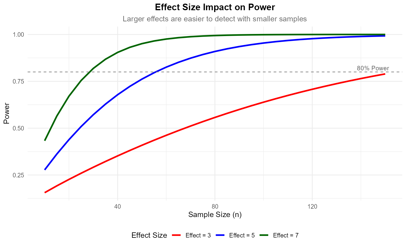
Fig. 10.10 Larger effect sizes lead to higher power for the same sample size.

Part (d): σ = 15 instead of σ = 10

Power decreases. Larger σ → larger SE → more overlap between H₀ and Hₐ distributions → harder to detect effects.

Part (e): Two-tailed to one-tailed test

Power increases. One-tailed test puts all α in one direction → lower critical value → easier to reject H₀ in that direction.

Part (f): Diminishing returns of sample size

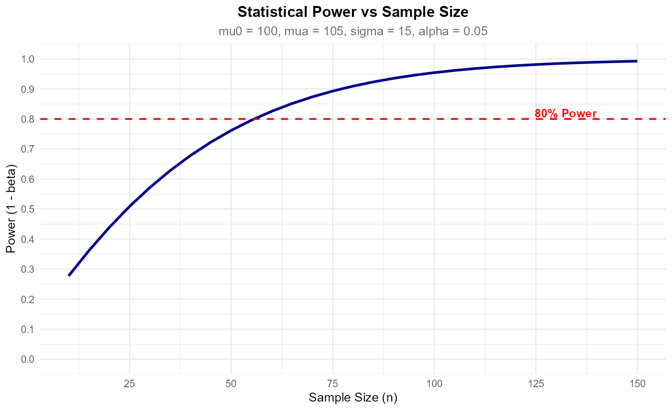
Fig. 10.11 Power increases with sample size but shows diminishing returns.

Power depends on SE = σ/√n. Because n is under a square root:

• Doubling n from 25 to 50 reduces SE by factor of √2 ≈ 1.41

• Doubling n from 100 to 200 also reduces SE by factor of √2 ≈ 1.41

But going from 25 to 50 is a smaller absolute increase (25) than 100 to 200 (100). The proportional improvement in power gets smaller as n increases, while the cost of additional samples stays constant or increases.

---

Exercise 8: True/False Conceptual Questions

Determine whether each statement is True or False. Provide a brief justification.

1. The significance level α is the probability of making a Type II error.

2. If we reject H₀, we have proven that H₀ is false.

3. A larger sample size reduces the probability of both Type I and Type II errors.

4. Power is the probability of correctly rejecting a false null hypothesis.

5. If a test has 90% power, there is a 10% chance of committing a Type I error.

6. The null hypothesis always contains an equality sign (=, ≤, or ≥).

Solution

Part (a): False

α is the probability of Type I error (rejecting a true H₀), not Type II error. Type II error probability is β.

Part (b): False

Rejecting H₀ means the data provides sufficient evidence against H₀, but it doesn’t prove H₀ is false. There’s always a chance (α) of incorrectly rejecting a true H₀.

Part (c): False

Larger sample size reduces Type II error (increases power), but Type I error probability is controlled at α regardless of sample size. α is set by the researcher, not determined by n.

Part (d): True

Power = 1 - β = P(reject H₀ | H₀ is false). It’s the probability of detecting a real effect.

Part (e): False

Power = 1 - β = 0.90 means β = 0.10, so there’s a 10% chance of Type II error (failing to reject a false H₀). Type I error probability is α, which is set separately.

Part (f): True

H₀ always includes an equality because it represents the status quo or baseline assumption. The three forms are: H₀: μ = μ₀, H₀: μ ≤ μ₀, or H₀: μ ≥ μ₀.

---

Exercise 9: Application - Clinical Trial Planning

A pharmaceutical company is planning a clinical trial to test whether a new drug reduces blood pressure. Historical data shows:

• Current treatment mean: μ₀ = 140 mmHg

• Population standard deviation: σ = 15 mmHg

• Clinically meaningful reduction: 5 mmHg (so μₐ = 135 mmHg)

• Desired power: 90%

• Significance level: α = 0.05

1. Write the hypotheses for this test.

2. Calculate the minimum sample size needed.

3. If the budget only allows for n = 50 patients, what power will the study have?

4. With n = 50, what is the minimum effect size detectable with 90% power?

5. Discuss the practical implications of these results for the study design.

Solution

Part (a): Hypotheses

Let μ = true mean blood pressure with new drug.

\[H_0: \mu \geq 140 \quad \text{vs} \quad H_a: \mu < 140\]

This is a lower-tailed test (testing if blood pressure is reduced).

Part (b): Required sample size for 90% power

For 90% power: \(z_{\beta} = z_{0.10} = 1.282\)

For α = 0.05 (one-sided): \(z_{\alpha} = z_{0.05} = 1.645\)

\[n = \left(\frac{(1.645 + 1.282) \times 15}{5}\right)^2 = \left(\frac{43.905}{5}\right)^2 = (8.781)^2 = 77.1\]

Minimum n = 78 patients

Part (c): Power with n = 50

\[SE = \frac{15}{\sqrt{50}} = 2.121\]

Cutoff (lower-tailed): \(\bar{x}_{cutoff} = 140 - 1.645 \times 2.121 = 136.51\)

Power = P(\(\bar{X} < 136.51\) | μ = 135):

\[P\left(Z < \frac{136.51 - 135}{2.121}\right) = P(Z < 0.712) = 0.762\]

Power ≈ 76.2% with n = 50

Part (d): Minimum detectable effect with n = 50 and 90% power

Rearranging the sample size formula:

\[|\mu_0 - \mu_a| = \frac{(z_{\alpha} + z_{\beta}) \sigma}{\sqrt{n}} = \frac{(1.645 + 1.282) \times 15}{\sqrt{50}} = \frac{43.905}{7.07} = 6.21\]

With n = 50, need at least a 6.2 mmHg reduction to achieve 90% power.

Part (e): Practical implications

1. Budget constraint is significant: With only 50 patients, power drops from 90% to 76%, meaning there’s nearly a 1-in-4 chance of missing a real 5 mmHg effect.

2. Recruitment challenge: Need 78 patients for adequate power—56% more than budget allows.

3. Effect size consideration: A 5 mmHg reduction may be clinically meaningful, but the study as designed can only reliably detect a 6+ mmHg effect.

4. Recommendations: - Seek additional funding for larger sample - Consider whether 76% power is acceptable given the study’s importance - Explore whether a larger effect size is realistic based on mechanism of action - Consider adaptive trial designs

R verification:

# Sample size
z_alpha <- qnorm(0.05, lower.tail = FALSE)  # 1.645
z_beta_90 <- qnorm(0.10, lower.tail = FALSE)  # 1.282
n_req <- ((z_alpha + z_beta_90) * 15 / 5)^2
ceiling(n_req)  # 78

# Power with n = 50
SE_50 <- 15 / sqrt(50)
cutoff <- 140 - z_alpha * SE_50
pnorm(cutoff, mean = 135, sd = SE_50)  # 0.762

# Minimum detectable effect
(z_alpha + z_beta_90) * 15 / sqrt(50)  # 6.21

---

10.1.7. Additional Practice Problems

True/False Questions (1 point each)

1. Type I error is also called a “false negative.”

   Ⓣ or Ⓕ

2. Increasing the significance level α increases statistical power.

   Ⓣ or Ⓕ

3. The alternative hypothesis is what we assume to be true until proven otherwise.

   Ⓣ or Ⓕ

4. Power and β are complements (Power = 1 - β).

   Ⓣ or Ⓕ

5. A two-tailed test has more power than a one-tailed test (same α).

   Ⓣ or Ⓕ

6. The sample size needed for a given power depends on the effect size.

   Ⓣ or Ⓕ

Multiple Choice Questions (2 points each)

7. A Type II error occurs when we:

   Ⓐ Reject H₀ when H₀ is true

   Ⓑ Fail to reject H₀ when H₀ is true

   Ⓒ Reject H₀ when H₀ is false

   Ⓓ Fail to reject H₀ when H₀ is false

8. If a test has power = 0.85, then β equals:

   Ⓐ 0.85

   Ⓑ 0.15

   Ⓒ 0.05

   Ⓓ Cannot be determined

9. Which action would INCREASE statistical power?

   Ⓐ Decrease sample size

   Ⓑ Decrease α from 0.05 to 0.01

   Ⓒ Increase population standard deviation

   Ⓓ Increase effect size

10. For the hypotheses H₀: μ ≤ 50 vs Hₐ: μ > 50, this is a:

    Ⓐ Lower-tailed test

    Ⓑ Upper-tailed test

    Ⓒ Two-tailed test

    Ⓓ None of the above

11. To achieve 80% power, \(z_{\beta}\) equals:

    Ⓐ 0.80

    Ⓑ 0.20

    Ⓒ 0.84

    Ⓓ 1.28

12. If the effect size doubles (with all else constant), the required sample size:

    Ⓐ Doubles

    Ⓑ Halves

    Ⓒ Quadruples

    Ⓓ Reduces to one-quarter

Answers to Practice Problems

True/False Answers:

1. False — Type I error is a “false positive” (incorrectly rejecting). Type II is the “false negative.”

2. True — Larger α makes it easier to reject H₀, increasing power (but also increasing Type I error risk).

3. False — The null hypothesis is assumed true until evidence suggests otherwise. The alternative is what we’re trying to find evidence for.

4. True — Power = P(reject H₀ | H₀ false) = 1 - P(fail to reject | H₀ false) = 1 - β.

5. False — A one-tailed test has more power (in the specified direction) because all of α is concentrated in one tail.

6. True — Larger effects are easier to detect, requiring smaller samples.

Multiple Choice Answers:

7. Ⓓ — Type II error = failing to reject a false H₀.

8. Ⓑ — Power = 1 - β, so 0.85 = 1 - β → β = 0.15.

9. Ⓓ — Larger effects are easier to detect, increasing power.

10. Ⓑ — Hₐ: μ > 50 is an upper-tailed (right-tailed) alternative.

11. Ⓒ — For 80% power, β = 0.20, and z₀.₂₀ = qnorm(0.20, lower.tail = FALSE) ≈ 0.84.

12. Ⓓ — n ∝ 1/(effect size)², so doubling effect size reduces n by factor of 4.