Slides 📊

Download Chapter 7 slides (PPTX)

7.2. Sampling Distribution for the Sample Mean

Having established that statistics are random variables with their own distributions, we now focus on the most important statistic in all of statistical inference: the sample mean \(\bar{X}\).

Road Map 🧭

• View the sample mean \(\bar{X}\) as a function of \(n\) independent and identically distributed random variables. Establish \(E[\bar{X}]\) and \(\text{Var}(\bar{X})\) in relation to the distributional properties of these building blocks.

• Define the standard deviation \(\sigma_{\bar{X}}\) of the sample mean as the standard error and understand how it is influenced by the population standard deviation and sample size.

7.2.1. A New Perspective on the Data-Generating Procedure

So far, we’ve pictured the sampling procedure as drawing individual datapoints \(n\) different times from a single random variable \(X\) (left of Fig. 7.3).

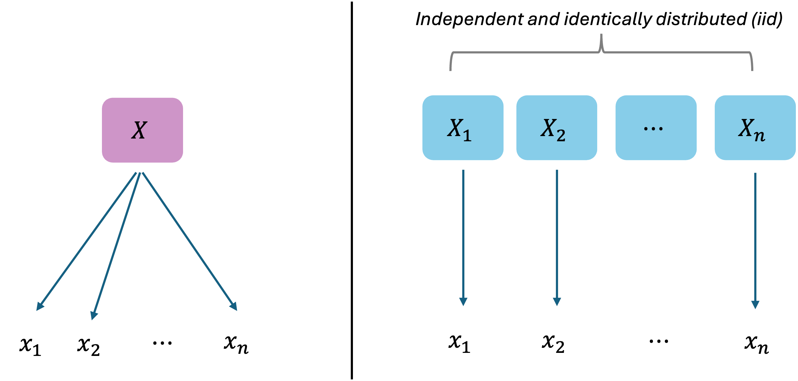
Fig. 7.3 Left represents how we used to think of the sampling procedure; we now think in the perspective on the right

For the formal understanding of the sampling distribution of \(\bar{X}\), we need to begin with a new perspective. Imagine that there are \(n\) independent and identically distributed (iid) copies of the population, \(X_1, X_2, \cdots, X_n\), and a sample is constructed by taking one data point from each copy (right of Fig. 7.3).

Through this shift, we can now express the sample mean \(\bar{X}\) as a function of \(n\) random variables:

\[\bar{X} = \frac{1}{n}\sum_{i=1}^n X_i\]

This allows us to break down the properties of the random variable \(\bar{X}\) in terms of its building blocks \(X_1, X_2, \cdots, X_n\), with which we are more familiar.

7.2.2. Visualizing Sampling Distributions

Let’s get a feel for how sampling distributions behave with a concrete visual example.

The Population: Exponential Distribution

Consider a population that follows an exponential distribution with parameter \(\lambda = 1\). Recall that this distribution is highly right-skewed, with most values bunched near 0 and a long tail extending to the right. The population mean is \(\mu = 1/\lambda = 1\), and the population standard deviation is \(\sigma = 1/\lambda = 1\).

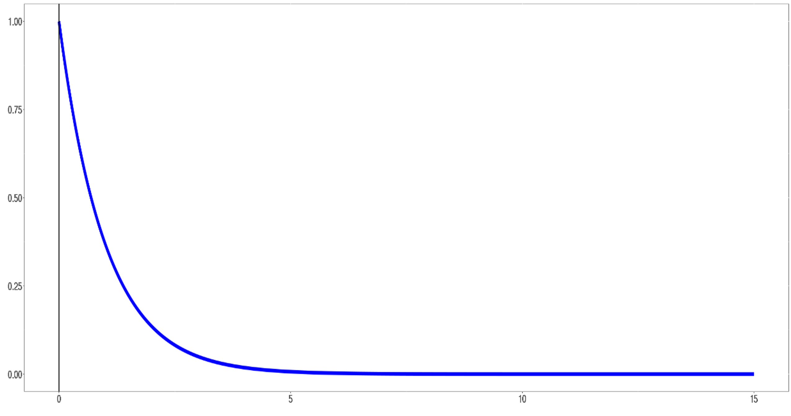
Fig. 7.4 The exponential population: highly right-skewed with mean \(\mu=1\)

When we conduct statistical inference in practice, we won’t know the population follows an exponential distribution or what its parameter value is. For now, we’ll assume this knowledge so we can compare our sample results to the known truth.

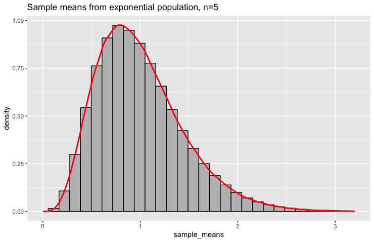
Sampling with n = 5

Let’s start by taking one sample of size \(n = 5\) from this population. The code below samples five numbers from the population and computes the average:

# Take one sample of size 5
sample1 <- rexp(5, rate = 1)
sample_mean1 <- mean(sample1)
# Result: 0.39

We repeat this process many times (num_samples). Each repetition samples a different set of five numbers and thus produces a different sample mean.

# Simulate the sampling distribution
num_samples <- 1000000
n <- 5
sample_means <- replicate(num_samples, mean(rexp(n, rate = 1)))

When we plot the distribution of these million sample means, we see something remarkable. The distribution no longer looks like the original exponential distribution. It’s still somewhat right-skewed, but the degree of skewness has diminished. The sample means cluster more tightly around the true population mean \(\mu=1\).

The Effect of Increasing Sample Size

Now let’s see what happens when we increase the sample size to \(n = 25\):

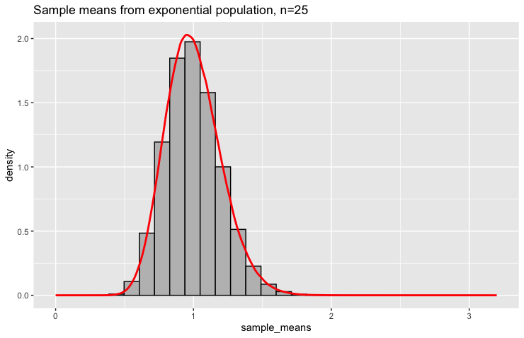
The transformation is dramatic. The sampling distribution is now roughly symmetric and centered around \(\mu = 1\). It bears little resemblance to the original exponential population. The sample means are much more concentrated around the true value—most fall between 0.5 and 1.5.

With \(n = 65\), the pattern becomes even more pronounced:

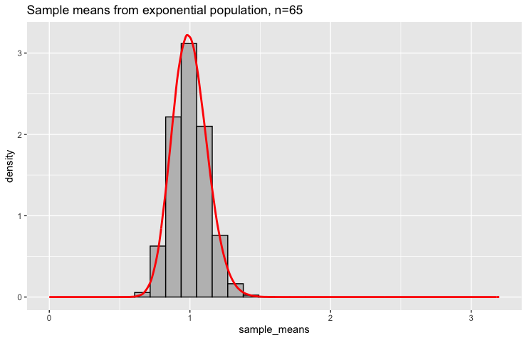
Now the distribution is highly concentrated around \(\mu = 1\) and appears very symmetric. The sample means rarely stray far from the true population mean.

Key Insights

1. The sample mean targets the population mean: All sampling distributions center around \(\mu = 1\), regardless of sample size.

2. Larger samples produce more precise estimates: As \(n\) increases, the sampling distribution becomes more concentrated around \(\mu\).

3. Shape changes with sample size: Even though the population is highly skewed, the sampling distribution becomes more symmetric as \(n\) increases.

4. The magic of averaging: By averaging multiple observations, we reduce the impact of extreme values and create estimators that behave better than individual observations.

7.2.3. Deriving the Mathematical Properties

To deepen our understanding of the sample mean’s behavior, we derive its key distributional properties: the mean, variance, and standard deviation. For clarity, all population parameters are written with a subscript \(X\) and all sampling distribution parameters with a subscript \(\bar{X}\).

A. Expected Value of the Sample Mean

\[\mu_{\bar{X}} = E[\bar{X}] = E\left[\frac{1}{n}\sum_{i=1}^n X_i\right] = \frac{1}{n} E\left[\sum_{i=1}^n X_i\right] = \frac{1}{n} \sum_{i=1}^n E[X_i]\]

Since all \(X_i\)’s come from the same distribution with \(E[X_i] = \mu_X\),

\[E[\bar{X}] = \frac{1}{n} \sum_{i=1}^n \mu_X = \frac{1}{n} \cdot n\mu_X = \mu_X\]

Unbiasedness of Sample Mean

The expected value of the sample mean equals the population mean (\(\mu_{\bar{X}} = \mu_X\)). When an estimator equals its target on average, we call it an unbiased estimator. Individual sample means may be too high or too low, but they center around the correct target.

B. Variance and Standard Error of the Sample Mean

\[\sigma^2_{\bar{X}}=\text{Var}(\bar{X}) =\text{Var}\left(\frac{1}{n}\sum_{i=1}^n X_i\right) = \frac{1}{n^2} \text{Var}\left(\sum_{i=1}^n X_i\right)\]

Since the \(X_i\)’s are independent, the variance of the sum equals the sum of the variances. Also, all \(X_i\)’s have the same variance \(\sigma_X^2\):

\[\text{Var}(\bar{X}) = \frac{1}{n^2} \sum_{i=1}^n\text{Var}(X_i) = \frac{1}{n^2} \cdot n\sigma^2_X = \frac{\sigma^2_X}{n}\]

We call the standard deviation of the sample mean the standard error. It is the positive square root of the variance of \(\bar{X}\).

\[\sigma_{\bar{X}} = \sqrt{\text{Var}(\bar{X})} = \frac{\sigma_X}{\sqrt{n}}\]

Understanding the Standard Error

For even modest sample sizes, sample means are much less variable than individual observations. With \(n = 25\), for example, the sample mean has standard error \(\frac{\sigma}{5}\), making it five times more precise than any single observation with standard deviation \(\sigma\).

This concentration effect explains why averaging is such a powerful statistical technique and why larger samples are usually better. By combining information from multiple observations, we create estimators that are more reliable than an individual measurement.

C. Summary of Basic Distributional Properties of \(\bar{X}\)

Name	Notation	Formula
Expected Value	\(E[\bar{X}]\) or \(\mu_{\bar{X}}\)	\(\mu_X\)
Variance	\(\text{Var}(\bar{X})\) or \(\sigma_{\bar{X}}^2\)	\(\frac{\sigma_X^2}{n}\)
Standard Error	\(\sigma_{\bar{X}}\)	\(\frac{\sigma_X}{\sqrt{n}}\)

Example💡: Maze Navigation Times

Researchers study how long it takes rats of a certain subspecies to navigate through a maze. Previous research suggests that navigation times have a mean \(\mu_X = 1.5\) minutes and a standard deviation \(\sigma_X=0.35\) minutes.

The researchers select five rats at random and want to understand the behavior of the average navigation time for their sample. What are the mean and the standard error of the sampling distribution for the sample mean?

Setting Up the Problem

We have:

• \(X_i\) are iid with \(E[X_i]=1.5\) and \(\text{Var}(X_i)=0.35^2\) for each \(i \in \{1,2,3,4,5\}\)

• \(n = 5\)

Mean of the Sample Mean

\[\mu_{\bar{X}} = \mu_X = 1.5 \text{ minutes}\]

Standard Error of the Sample Mean

\[\sigma_{\bar{X}} = \frac{\sigma}{\sqrt{n}} = \frac{0.35}{\sqrt{5}} = \frac{0.35}{2.236} = 0.1565 \text{ minutes}\]

7.2.4. The Special Case: Normal Populations

While our mathematical results apply to any population with finite mean and variance, there’s one special case where we can say much more about the shape of the sampling distribution: when the population follows a normal distribution.

Linear Combinations of Normal Random Variables

A key property of normal distributions is that linear combinations of normal random variables are themselves normal. That is, if \(X\) and \(Y\) are normal random variables, then any linear combination of the form \(aX + bY + c\) is also normal.

The sample mean is exactly such a linear combination:

\[\bar{X} = \frac{1}{n}X_1 + \frac{1}{n}X_2 + \cdots + \frac{1}{n}X_n\]

The Exact Distribution of \(\bar{X}\) from Normal Population

If \(X_1, X_2, \cdots, X_n\) are iid from a normal distribution with mean \(\mu_X\) and standard deviation \(\sigma_X\), then:

\[\bar{X} \sim N\left(\mu_X, \frac{\sigma_X^2}{n}\right) \quad \text{ or equivalently,} \quad \bar{X} \sim N\left(\mu_X, \frac{\sigma_X}{\sqrt{n}}\right)\]

This result is remarkable because it tells us the exact sampling distribution, not just its mean and variance.

Example💡: Maze Navigation Times, Continued

Researchers study how long it takes rats of a certain subspecies to navigate through a maze. In addition to the parameters \(\mu = 1.5\) minutes and \(\sigma = 0.35\) minutes, it is known that the population of navigation times follow normal distribution.

Setting Up the Problem

From the previous example, we have

• \(\mu_{\bar{X}} = 1.5\)

• \(\sigma_{\bar{X}} = 0.1565\)

Since the population follows normal distribution, the sampling distribution for the sample mean must also be normal. We have:

\[\bar{X} \sim N(\mu_{\bar{X}} = 1.5, \sigma^2_{\bar{X}} = 0.1565^2)\]

Computing Probabilities

What’s the probability that the average navigation time for five rats exceeds 1.75 minutes?

We need to find \(P(\bar{X} > 1.75)\). Since \(\bar{X} \sim N(1.5, 0.1565^2)\), we use the standardization technique and the Z-table (or a statistical software) to compute:

\[\begin{split}&P(\bar{X} > 1.75) = P\left(\frac{\bar{X} - 1.5}{0.1565} > \frac{1.75 - 1.5}{0.1565}\right)\\ &= P(Z > 1.60) = 1 - \Phi(1.60) = 1 - 0.9452 = 0.0548\end{split}\]

There’s 0.0548 probability that the average navigation time for five randomly selected rats will exceed 1.75 minutes.

7.2.5. Additional Example: Quality Control in Manufacturing

Let us conclude this section by solving a problem applying the CLT to decision-making in in quality control.

Example 💡: Quality Control in Manufacturing

The Bulls Eye Production company manufactures a number of high precision tools. Under the usual production process, one of these tools has a mean diameter of 5mm. The measurement varies normally aroud this mean, with standard deviation of 0.5mm.

However, the machine will need to be frequently recalibrated due to the strenuous operating conditions. Recalibration is required anytime the difference between the observed sample mean diameter and the ideal diameter is too large. “Large” is measured probabilistically; if the probability of the deviation is rarer than 0.05, then the difference is considered too large.

A random sample of size 64 is taken to assess the need for recalibration. It is found that the average diameter of the sample is 4.85mm. Is recalibration necessary?

Setting Up the Problem

It is given that

• \(n=64\)

• \(\mu_X = 5\) and \(\sigma_X = 0.5\)

• The population is normally distributed.

• The sample is randomly collected from the same population, which allows us to assume the iid condition.

• A single realization from \(\bar{X}\) has value \(\bar{x} = 4.85\).

Solving the Problem

We must compute a probability representing how rare the current difference \(|\bar{x}-\mu_X|\) is when compared with the general behavior of \(|\bar{X}-\mu_X|\).

\[\begin{split}&P(|\bar{X}-\mu_X| > |\bar{x}-\mu_X|)\\ &= P(|\bar{X}-\mu_X| > |4.85-5|)\\ &=P(\Bigg|\frac{\bar{X}-\mu_X}{\sigma_X/\sqrt{n}}\Bigg| > \frac{|4.85-5|}{0.5/\sqrt{64}})\\ &=P(|Z| > 2.4) = P(Z > 2.4) + P(Z < -2.4)\\ &=\underbrace{2P(Z < -2.4)}_{\text{by symmetry around } 0} = 0.0164\end{split}\]

The probability of seeing an even larger difference than the current observation is only 0.0164, which is smaller than 0.05. Therefore, the machine must be recalibrated.

7.2.6. Bringing It All Together

Key Takeaways 📝

1. The sample mean \(\bar{X}\) is a random variable. Its probability distribution is called the sampling distribution of the sample mean.

2. If the population has mean \(\mu_X\) and variance \(\sigma_X^2\), then \(\mu_{\bar{X}} = E[\bar{X}] = \mu_X\) and \(\sigma^2_{\bar{X}} = Var(\bar{X}) = \sigma_X^2/n\).

3. If the population has a distribution \(N(\mu_X, \sigma_X^2)\), then the sampling distribution of \(\bar{X}\) is completely known: \(\bar{X} \sim N(\mu_X, \sigma_X^2/n)\).

7.2.7. Exercises

These exercises develop your skills in working with the sampling distribution of the sample mean, including computing the expected value and standard error, finding probabilities when the population is normal, and determining sample sizes for desired precision.

Key Formulas

For a random sample of size \(n\) from a population with mean \(\mu\) and standard deviation \(\sigma\):

• Expected Value: \(E[\bar{X}] = \mu_{\bar{X}} = \mu\)

• Variance: \(\text{Var}(\bar{X}) = \sigma^2_{\bar{X}} = \frac{\sigma^2}{n}\)

• Standard Error: \(\sigma_{\bar{X}} = \frac{\sigma}{\sqrt{n}}\)

Special Case — Normal Population: If the population is \(N(\mu, \sigma^2)\), then:

\[\bar{X} \sim N\left(\mu, \frac{\sigma^2}{n}\right)\]

R Functions for Normal Probabilities and Quantiles

For \(\bar{X} \sim N(\mu_{\bar{X}}, \sigma_{\bar{X}})\):

# Probability calculations
pnorm(x, mean = mu, sd = sigma_xbar)               # P(X̄ ≤ x)
pnorm(x, mean = mu, sd = sigma_xbar, lower.tail = FALSE)  # P(X̄ > x)

# Quantile (inverse CDF) - find x such that P(X̄ ≤ x) = p
qnorm(p, mean = mu, sd = sigma_xbar)

Example: For \(\bar{X} \sim N(100, 4)\) (mean 100, SD 2):

pnorm(102, mean = 100, sd = 2)                # P(X̄ ≤ 102) = 0.8413
pnorm(102, mean = 100, sd = 2, lower.tail = FALSE)  # P(X̄ > 102) = 0.1587
qnorm(0.95, mean = 100, sd = 2)              # 95th percentile = 103.29

Important Note

The formulas for \(E[\bar{X}]\) and \(\text{Var}(\bar{X})\) hold for any population with finite mean and variance. However, we can only determine the exact shape of the sampling distribution when the population is normal. For non-normal populations, the Central Limit Theorem (Section 7.3) provides an approximation for large samples.

Exercise 1: Basic Properties of the Sampling Distribution

The tensile strength of a certain type of steel cable is normally distributed with mean \(\mu = 850\) pounds and standard deviation \(\sigma = 40\) pounds. A quality control engineer selects a random sample of \(n = 16\) cables for testing.

1. What is the expected value of the sample mean tensile strength?

2. What is the standard error of the sample mean?

3. What is the complete sampling distribution of \(\bar{X}\)?

4. Compare the standard error to the population standard deviation. What does this tell you about the precision of the sample mean versus a single observation?

Solution

Let \(X\) = tensile strength (pounds), where \(X \sim N(\mu = 850, \sigma = 40)\) and \(n = 16\).

Part (a): Expected value of X̄

\[E[\bar{X}] = \mu = 850 \text{ pounds}\]

The sample mean is centered at the population mean.

Part (b): Standard error

\[\sigma_{\bar{X}} = \frac{\sigma}{\sqrt{n}} = \frac{40}{\sqrt{16}} = \frac{40}{4} = 10 \text{ pounds}\]

Part (c): Complete sampling distribution

Since the population is normal, the sampling distribution is also normal:

\[\bar{X} \sim N\left(850, 10^2\right) \quad \text{or equivalently} \quad \bar{X} \sim N(850, 100)\]

Part (d): Precision comparison

The standard error (10 pounds) is one-fourth of the population standard deviation (40 pounds). This means the sample mean of 16 cables is 4 times more precise than a single cable measurement. Averaging reduces variability by a factor of \(\sqrt{n} = \sqrt{16} = 4\).

---

Exercise 2: Probability Calculations with Normal Population

The diameter of ball bearings produced by a machine is normally distributed with mean \(\mu = 5.00\) mm and standard deviation \(\sigma = 0.10\) mm. A random sample of \(n = 25\) ball bearings is selected.

1. Find \(P(\bar{X} > 5.03)\).

2. Find \(P(\bar{X} < 4.96)\).

3. Find \(P(4.97 < \bar{X} < 5.03)\).

4. Find the value \(c\) such that \(P(\bar{X} > c) = 0.10\).

Solution

Let \(X\) = diameter (mm), where \(X \sim N(5.00, 0.10^2)\) and \(n = 25\).

First, find the sampling distribution parameters:

• \(E[\bar{X}] = 5.00\) mm

• \(\sigma_{\bar{X}} = \frac{0.10}{\sqrt{25}} = \frac{0.10}{5} = 0.02\) mm

Since the population is normal: \(\bar{X} \sim N(5.00, 0.02^2)\).

Part (a): P(X̄ > 5.03)

\[P(\bar{X} > 5.03) = P\left(Z > \frac{5.03 - 5.00}{0.02}\right) = P(Z > 1.50)\]

\[= 1 - \Phi(1.50) = 1 - 0.9332 = 0.0668\]

R verification:

pnorm(5.03, mean = 5.00, sd = 0.02, lower.tail = FALSE)
# [1] 0.0668

Part (b): P(X̄ < 4.96)

\[P(\bar{X} < 4.96) = P\left(Z < \frac{4.96 - 5.00}{0.02}\right) = P(Z < -2.00)\]

\[= \Phi(-2.00) = 0.0228\]

R verification:

pnorm(4.96, mean = 5.00, sd = 0.02)
# [1] 0.0228

Part (c): P(4.97 < X̄ < 5.03)

\[P(4.97 < \bar{X} < 5.03) = P\left(\frac{4.97 - 5.00}{0.02} < Z < \frac{5.03 - 5.00}{0.02}\right)\]

\[= P(-1.50 < Z < 1.50) = \Phi(1.50) - \Phi(-1.50) = 0.9332 - 0.0668 = 0.8664\]

R verification:

pnorm(5.03, mean = 5.00, sd = 0.02) - pnorm(4.97, mean = 5.00, sd = 0.02)
# [1] 0.8664

Part (d): Find c such that P(X̄ > c) = 0.10

We need the 90th percentile of \(\bar{X}\).

From the Z-table: \(\Phi(1.28) = 0.8997 \approx 0.90\), so \(z_{0.90} \approx 1.28\).

\[c = \mu + z_{0.90} \cdot \sigma_{\bar{X}} = 5.00 + 1.28(0.02) = 5.00 + 0.0256 = 5.026 \text{ mm}\]

R verification:

qnorm(0.90, mean = 5.00, sd = 0.02)
# [1] 5.0256

---

Exercise 3: Standard Error and Sample Size

A biomedical engineer is measuring the response time of a neural sensor. The population standard deviation is known to be \(\sigma = 8\) milliseconds.

1. If a sample of \(n = 16\) measurements is taken, what is the standard error of \(\bar{X}\)?

2. If the sample size is increased to \(n = 64\), what is the new standard error?

3. By what factor did the standard error decrease when the sample size was quadrupled?

4. What sample size is needed to achieve a standard error of at most 1 millisecond?

5. A colleague claims that doubling the sample size will cut the standard error in half. Is this correct? Explain.

Solution

Given: \(\sigma = 8\) ms.

Part (a): SE with n = 16

\[\sigma_{\bar{X}} = \frac{8}{\sqrt{16}} = \frac{8}{4} = 2 \text{ ms}\]

Part (b): SE with n = 64

\[\sigma_{\bar{X}} = \frac{8}{\sqrt{64}} = \frac{8}{8} = 1 \text{ ms}\]

Part (c): Factor of decrease

The standard error decreased from 2 ms to 1 ms, a factor of 2.

When sample size quadruples (×4), the standard error decreases by \(\sqrt{4} = 2\).

In general: \(\frac{\text{SE}_{\text{old}}}{\text{SE}_{\text{new}}} = \frac{\sigma/\sqrt{n_{\text{old}}}}{\sigma/\sqrt{n_{\text{new}}}} = \sqrt{\frac{n_{\text{new}}}{n_{\text{old}}}} = \sqrt{\frac{64}{16}} = 2\).

Part (d): Sample size for SE ≤ 1 ms

We need \(\frac{\sigma}{\sqrt{n}} \leq 1\), which gives \(\sqrt{n} \geq \sigma = 8\), so \(n \geq 64\).

Minimum sample size: n = 64.

Part (e): Does doubling n halve the SE?

No, this is incorrect. Doubling the sample size reduces the standard error by a factor of \(\sqrt{2} \approx 1.41\), not 2.

If \(n \to 2n\), then \(\sigma_{\bar{X}} = \frac{\sigma}{\sqrt{n}} \to \frac{\sigma}{\sqrt{2n}} = \frac{\sigma}{\sqrt{2}\sqrt{n}}\).

To halve the standard error, you must quadruple the sample size.

---

Exercise 4: Comparing Individual Observations to Sample Means

CPU processing times for a certain task are normally distributed with mean \(\mu = 120\) ms and standard deviation \(\sigma = 15\) ms.

1. What is the probability that a single randomly selected task takes more than 130 ms?

2. What is the probability that the average of \(n = 9\) randomly selected tasks exceeds 130 ms?

3. What is the probability that the average of \(n = 36\) randomly selected tasks exceeds 130 ms?

4. Explain why the probabilities in (a), (b), and (c) are different.

Solution

Let \(X\) = processing time (ms), where \(X \sim N(120, 15^2)\).

Part (a): Single observation, P(X > 130)

For a single observation, we use the population distribution directly:

\[P(X > 130) = P\left(Z > \frac{130 - 120}{15}\right) = P(Z > 0.67)\]

\[= 1 - \Phi(0.67) = 1 - 0.7486 = 0.2514\]

Part (b): Sample mean with n = 9

\(\sigma_{\bar{X}} = \frac{15}{\sqrt{9}} = 5\) ms, and \(\bar{X} \sim N(120, 5^2)\).

\[P(\bar{X} > 130) = P\left(Z > \frac{130 - 120}{5}\right) = P(Z > 2.00)\]

\[= 1 - \Phi(2.00) = 1 - 0.9772 = 0.0228\]

Part (c): Sample mean with n = 36

\(\sigma_{\bar{X}} = \frac{15}{\sqrt{36}} = 2.5\) ms, and \(\bar{X} \sim N(120, 2.5^2)\).

\[P(\bar{X} > 130) = P\left(Z > \frac{130 - 120}{2.5}\right) = P(Z > 4.00)\]

\[= 1 - \Phi(4.00) \approx 1 - 0.99997 \approx 0.00003\]

R verification:

# Part (a): Single observation
pnorm(130, mean = 120, sd = 15, lower.tail = FALSE)
# [1] 0.2525

# Part (b): Sample mean, n = 9
pnorm(130, mean = 120, sd = 15/sqrt(9), lower.tail = FALSE)
# [1] 0.0228

# Part (c): Sample mean, n = 36
pnorm(130, mean = 120, sd = 15/sqrt(36), lower.tail = FALSE)
# [1] 3.167e-05

Part (d): Explanation

The probabilities decrease dramatically as sample size increases because:

• Individual observations have high variability (\(\sigma = 15\) ms)

• Sample means have reduced variability (\(\sigma_{\bar{X}} = \sigma/\sqrt{n}\))

• Larger samples produce means that cluster more tightly around \(\mu = 120\)

A single observation exceeding 130 ms is fairly common (25% chance), but a sample mean of 36 observations exceeding 130 ms is extremely rare (0.003% chance) because extreme values in individual observations tend to cancel out when averaging.

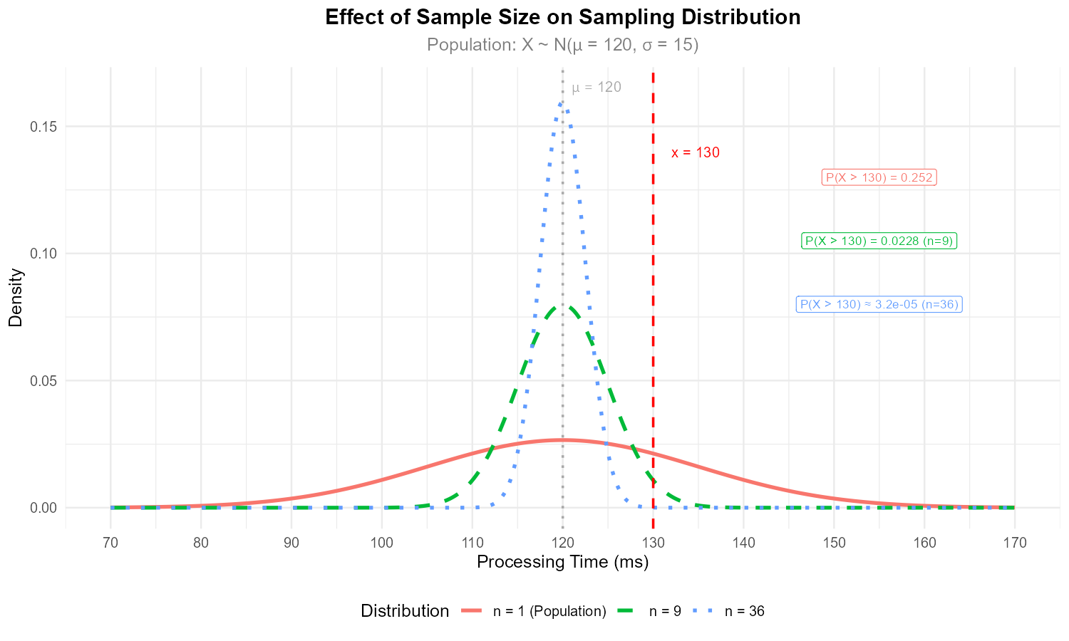
Fig. 7.5 As sample size increases, the sampling distribution becomes more concentrated around μ = 120.

---

Exercise 5: Quality Control Application

A pharmaceutical company fills capsules with an active ingredient. The filling process is normally distributed with a target mean of \(\mu = 500\) mg and standard deviation \(\sigma = 12\) mg. To monitor quality, a random sample of \(n = 9\) capsules is tested each hour.

1. What is the sampling distribution of \(\bar{X}\)?

2. If the process is operating correctly (at \(\mu = 500\)), what is the probability that the sample mean falls between 492 mg and 508 mg?

3. The quality control protocol triggers an investigation if \(\bar{X}\) falls outside the interval \([492, 508]\). What is the probability of triggering an investigation when the process is operating correctly? (This is called a “false alarm” rate.)

4. Suppose the process drifts so that \(\mu = 506\) mg (but \(\sigma\) remains 12 mg). What is the probability that \(\bar{X}\) falls within \([492, 508]\)? (This represents failing to detect a problem.)

Solution

Given: Target \(\mu = 500\) mg, \(\sigma = 12\) mg, \(n = 9\).

Part (a): Sampling distribution

\[\sigma_{\bar{X}} = \frac{12}{\sqrt{9}} = 4 \text{ mg}\]

Since the population is normal:

\[\bar{X} \sim N(500, 4^2) \quad \text{or} \quad \bar{X} \sim N(500, 16)\]

Part (b): P(492 < X̄ < 508) when μ = 500

\[P(492 < \bar{X} < 508) = P\left(\frac{492 - 500}{4} < Z < \frac{508 - 500}{4}\right)\]

\[= P(-2.00 < Z < 2.00) = \Phi(2.00) - \Phi(-2.00) = 0.9772 - 0.0228 = 0.9544\]

Part (c): False alarm rate

The probability of triggering an investigation when the process is correct:

\[P(\bar{X} < 492 \text{ or } \bar{X} > 508) = 1 - P(492 < \bar{X} < 508) = 1 - 0.9544 = 0.0456\]

About 4.56% of the time, an investigation will be triggered even when the process is operating correctly.

Part (d): P(492 < X̄ < 508) when μ = 506 (process drift)

Now \(\bar{X} \sim N(506, 4^2)\):

\[P(492 < \bar{X} < 508) = P\left(\frac{492 - 506}{4} < Z < \frac{508 - 506}{4}\right)\]

\[= P(-3.50 < Z < 0.50) = \Phi(0.50) - \Phi(-3.50)\]

\[= 0.6915 - 0.0002 = 0.6913\]

There is about a 69% probability that the sample mean falls in the acceptable range even though the process has drifted. This means the protocol fails to detect the problem about 69% of the time—a concern for quality control effectiveness.

R verification:

se <- 12/sqrt(9)  # Standard error = 4

# Part (b): P(492 < X̄ < 508) when μ = 500
pnorm(508, mean = 500, sd = se) - pnorm(492, mean = 500, sd = se)
# [1] 0.9545

# Part (c): False alarm rate
1 - (pnorm(508, mean = 500, sd = se) - pnorm(492, mean = 500, sd = se))
# [1] 0.0455

# Part (d): P(492 < X̄ < 508) when μ = 506
pnorm(508, mean = 506, sd = se) - pnorm(492, mean = 506, sd = se)
# [1] 0.6915

---

Exercise 6: Working Backward — Finding Population Parameters

For a normally distributed population, a sample of size \(n = 25\) yields a sampling distribution for \(\bar{X}\) with standard error \(\sigma_{\bar{X}} = 3\).

1. What is the population standard deviation \(\sigma\)?

2. If the sample size were increased to \(n = 100\), what would be the new standard error?

3. If the population standard deviation were actually \(\sigma = 20\), what sample size would be needed to achieve the original standard error of 3?

Solution

Part (a): Find σ from SE

Given: \(\sigma_{\bar{X}} = 3\) and \(n = 25\).

\[\sigma_{\bar{X}} = \frac{\sigma}{\sqrt{n}} \implies 3 = \frac{\sigma}{\sqrt{25}} = \frac{\sigma}{5}\]

\[\sigma = 3 \times 5 = 15\]

Part (b): New SE with n = 100

\[\sigma_{\bar{X}} = \frac{15}{\sqrt{100}} = \frac{15}{10} = 1.5\]

Part (c): Sample size for SE = 3 when σ = 20

\[3 = \frac{20}{\sqrt{n}} \implies \sqrt{n} = \frac{20}{3} \implies n = \left(\frac{20}{3}\right)^2 = \frac{400}{9} = 44.44\]

Since sample size must be a whole number, we need \(n \geq 45\) to achieve a standard error of at most 3.

---

Exercise 7: Symmetric Probability Bounds

The weight of packages shipped by an e-commerce company is normally distributed with mean \(\mu = 2.5\) kg and standard deviation \(\sigma = 0.4\) kg. For a random sample of \(n = 16\) packages:

1. Find the value \(d\) such that \(P(|\bar{X} - \mu| < d) = 0.95\).

2. Interpret this result in context.

3. How would \(d\) change if the sample size were increased to \(n = 64\)?

Solution

Given: \(\mu = 2.5\) kg, \(\sigma = 0.4\) kg, \(n = 16\).

First, find the standard error:

\[\sigma_{\bar{X}} = \frac{0.4}{\sqrt{16}} = 0.1 \text{ kg}\]

Part (a): Find d such that P(|X̄ − μ| < d) = 0.95

We need \(P(-d < \bar{X} - \mu < d) = 0.95\).

Standardizing:

\[P\left(-\frac{d}{\sigma_{\bar{X}}} < Z < \frac{d}{\sigma_{\bar{X}}}\right) = 0.95\]

For this symmetric interval around 0, we need \(\frac{d}{\sigma_{\bar{X}}} = z_{0.975}\).

From the Z-table: \(z_{0.975} = 1.96\).

\[d = 1.96 \times \sigma_{\bar{X}} = 1.96 \times 0.1 = 0.196 \text{ kg}\]

R verification:

# Find z_{0.975}
qnorm(0.975)
# [1] 1.96

# Calculate d
1.96 * 0.1
# [1] 0.196

Part (b): Interpretation

There is a 95% probability that the sample mean weight of 16 packages will be within 0.196 kg (about 196 grams) of the true population mean. In other words, 95% of all possible sample means will fall in the interval \([2.304, 2.696]\) kg.

Part (c): Effect of increasing n to 64

New standard error:

\[\sigma_{\bar{X}} = \frac{0.4}{\sqrt{64}} = 0.05 \text{ kg}\]

New \(d\):

\[d = 1.96 \times 0.05 = 0.098 \text{ kg}\]

The bound halves (from 0.196 to 0.098 kg) when sample size quadruples. Larger samples produce sample means that stay closer to the population mean.

---

Exercise 8: The iid Framework

Consider the sampling framework where \(X_1, X_2, \ldots, X_n\) are independent and identically distributed (iid) random variables, each with mean \(\mu\) and variance \(\sigma^2\).

1. Explain in your own words what “independent” means in this context.

2. Explain what “identically distributed” means in this context.

3. Why is the iid assumption important for deriving the variance formula \(\text{Var}(\bar{X}) = \sigma^2/n\)?

4. Give an example of a sampling scenario where the iid assumption might be violated.

Solution

Part (a): Independence

“Independent” means that the value of one observation does not affect or provide information about the values of other observations. Mathematically, knowing \(X_1 = x_1\) does not change the probability distribution of \(X_2, X_3, \ldots, X_n\).

In practice, this typically requires random sampling where each unit is selected without regard to other selected units.

Part (b): Identically distributed

“Identically distributed” means all observations come from the same probability distribution—they have the same mean \(\mu\), same variance \(\sigma^2\), and same distributional shape. This ensures we’re sampling from a single, well-defined population.

Part (c): Importance of iid for variance formula

The derivation of \(\text{Var}(\bar{X}) = \sigma^2/n\) relies on:

1. Independence: This allows us to write \(\text{Var}(X_1 + X_2 + \cdots + X_n) = \text{Var}(X_1) + \text{Var}(X_2) + \cdots + \text{Var}(X_n)\). Without independence, we would need to include covariance terms.

2. Identical distribution: This ensures each \(\text{Var}(X_i) = \sigma^2\), so the sum of variances equals \(n\sigma^2\).

Together, these give \(\text{Var}(\bar{X}) = \frac{1}{n^2} \cdot n\sigma^2 = \frac{\sigma^2}{n}\).

Part (d): Violation example

Cluster sampling: If we sample households and then measure all individuals within each household, observations within the same household are likely correlated (not independent)—family members may share similar characteristics.

Time series data: Measurements taken over time (e.g., daily stock prices) often exhibit dependence, where today’s value is related to yesterday’s value.

Sampling without replacement from a small population: If the population is small relative to the sample, observations are not truly independent because removing one unit changes the composition of remaining units.

---

Exercise 9: Comprehensive Application — Engine Performance

A mechanical engineer is testing fuel efficiency of a new engine design. Based on extensive prior testing, fuel efficiency (in miles per gallon) is known to be normally distributed with mean \(\mu = 32\) mpg and standard deviation \(\sigma = 3\) mpg.

1. For a single test run, what is the probability of observing fuel efficiency above 35 mpg?

2. The engineer conducts \(n = 12\) test runs and computes the sample mean. What is the distribution of \(\bar{X}\)?

3. Find \(P(\bar{X} > 33)\) for the sample of 12 runs.

4. Find the 5th and 95th percentiles of the sampling distribution of \(\bar{X}\).

5. The engineer wants the standard error to be at most 0.5 mpg. How many test runs are needed?

6. If the engineer observes \(\bar{x} = 34.2\) mpg from 12 test runs, should this be considered unusual? Calculate the probability of observing a sample mean at least this far from \(\mu = 32\).

Solution

Given: \(X \sim N(\mu = 32, \sigma = 3)\) mpg.

Part (a): P(X > 35) for single observation

\[P(X > 35) = P\left(Z > \frac{35 - 32}{3}\right) = P(Z > 1.00) = 1 - 0.8413 = 0.1587\]

Part (b): Distribution of X̄ with n = 12

\[\sigma_{\bar{X}} = \frac{3}{\sqrt{12}} = \frac{3}{3.464} = 0.866 \text{ mpg}\]

\[\bar{X} \sim N(32, 0.866^2) \quad \text{or} \quad \bar{X} \sim N(32, 0.75)\]

Part (c): P(X̄ > 33)

\[P(\bar{X} > 33) = P\left(Z > \frac{33 - 32}{0.866}\right) = P(Z > 1.15)\]

\[= 1 - \Phi(1.15) = 1 - 0.8749 = 0.1251\]

Part (d): 5th and 95th percentiles

From Z-table: \(z_{0.05} = -1.645\) and \(z_{0.95} = 1.645\).

5th percentile:

\[\bar{x}_{0.05} = \mu + z_{0.05} \cdot \sigma_{\bar{X}} = 32 + (-1.645)(0.866) = 32 - 1.42 = 30.58 \text{ mpg}\]

95th percentile:

\[\bar{x}_{0.95} = 32 + (1.645)(0.866) = 32 + 1.42 = 33.42 \text{ mpg}\]

90% of sample means will fall between 30.58 and 33.42 mpg.

Part (e): Sample size for SE ≤ 0.5 mpg

\[\frac{\sigma}{\sqrt{n}} \leq 0.5 \implies \frac{3}{\sqrt{n}} \leq 0.5 \implies \sqrt{n} \geq 6 \implies n \geq 36\]

At least 36 test runs are needed.

Part (f): Is x̄ = 34.2 unusual?

The observed sample mean is 34.2 − 32 = 2.2 mpg away from \(\mu\).

We compute \(P(|\bar{X} - 32| \geq 2.2)\):

\[P(|\bar{X} - 32| \geq 2.2) = P(\bar{X} \leq 29.8) + P(\bar{X} \geq 34.2)\]

\[= P\left(Z \leq \frac{29.8 - 32}{0.866}\right) + P\left(Z \geq \frac{34.2 - 32}{0.866}\right)\]

\[= P(Z \leq -2.54) + P(Z \geq 2.54) = 2 \times P(Z \leq -2.54)\]

\[= 2 \times 0.0055 = 0.011\]

Yes, this is unusual. There is only about a 1.1% probability of observing a sample mean at least 2.2 mpg away from the true mean if \(\mu = 32\). This result suggests the engine may actually have different fuel efficiency than assumed, or something unusual occurred during testing.

R verification:

mu <- 32
sigma <- 3
n <- 12
se <- sigma / sqrt(n)  # 0.866

# Part (a): Single observation P(X > 35)
pnorm(35, mean = mu, sd = sigma, lower.tail = FALSE)
# [1] 0.1587

# Part (c): P(X̄ > 33)
pnorm(33, mean = mu, sd = se, lower.tail = FALSE)
# [1] 0.1241

# Part (d): 5th and 95th percentiles
qnorm(0.05, mean = mu, sd = se)
# [1] 30.58
qnorm(0.95, mean = mu, sd = se)
# [1] 33.42

# Part (f): Two-tailed probability
2 * pnorm(29.8, mean = mu, sd = se)
# [1] 0.0110

---

7.2.8. Additional Practice Problems

True/False Questions (1 point each)

1. The expected value of the sample mean equals the population mean for any sample size.

   Ⓣ or Ⓕ

2. The standard error of \(\bar{X}\) increases as sample size increases.

   Ⓣ or Ⓕ

3. If the population is normally distributed, then \(\bar{X}\) is exactly normally distributed regardless of sample size.

   Ⓣ or Ⓕ

4. Doubling the sample size will cut the standard error in half.

   Ⓣ or Ⓕ

5. The variance of the sample mean is \(\sigma^2/n\), where \(\sigma^2\) is the population variance.

   Ⓣ or Ⓕ

6. The sampling distribution of \(\bar{X}\) has the same standard deviation as the population.

   Ⓣ or Ⓕ

Multiple Choice Questions (2 points each)

7. A population has \(\mu = 100\) and \(\sigma = 20\). For samples of size \(n = 25\), the standard error of \(\bar{X}\) is:

   Ⓐ 0.8

   Ⓑ 4

   Ⓒ 20

   Ⓓ 100

8. If the population is normal with \(\mu = 50\) and \(\sigma = 10\), and \(n = 4\), then \(\bar{X}\) follows:

   Ⓐ \(N(50, 100)\)

   Ⓑ \(N(50, 25)\)

   Ⓒ \(N(50, 10)\)

   Ⓓ \(N(12.5, 2.5)\)

9. To reduce the standard error by half, you must:

   Ⓐ Double the sample size

   Ⓑ Triple the sample size

   Ⓒ Quadruple the sample size

   Ⓓ Halve the population standard deviation

10. For a normal population with \(\sigma = 12\), what sample size gives \(\sigma_{\bar{X}} = 2\)?

    Ⓐ 6

    Ⓑ 24

    Ⓒ 36

    Ⓓ 144

11. If \(X \sim N(80, 16)\) (variance = 16), and \(n = 4\), then \(P(\bar{X} > 82)\) equals:

    Ⓐ \(P(Z > 0.5)\)

    Ⓑ \(P(Z > 1)\)

    Ⓒ \(P(Z > 2)\)

    Ⓓ \(P(Z > 4)\)

12. The formula \(\text{Var}(\bar{X}) = \sigma^2/n\) requires which assumption?

    Ⓐ The population must be normal

    Ⓑ The sample size must be at least 30

    Ⓒ The observations must be independent

    Ⓓ The population mean must be known

Answers to Practice Problems

True/False Answers:

1. True — \(E[\bar{X}] = \mu\) always holds when sampling from a population with mean \(\mu\).

2. False — The standard error \(\sigma/\sqrt{n}\) decreases as \(n\) increases.

3. True — Linear combinations of normal random variables are normal, so \(\bar{X}\) is exactly normal when the population is normal.

4. False — Doubling \(n\) reduces SE by factor of \(\sqrt{2} \approx 1.41\), not 2. To halve SE, you must quadruple \(n\).

5. True — This is the variance formula for the sample mean.

6. False — The sampling distribution has standard deviation \(\sigma/\sqrt{n}\), which is smaller than \(\sigma\) when \(n > 1\).

Multiple Choice Answers:

7. Ⓑ — \(\sigma_{\bar{X}} = 20/\sqrt{25} = 20/5 = 4\).

8. Ⓑ — \(\bar{X} \sim N(\mu, \sigma^2/n) = N(50, 100/4) = N(50, 25)\).

9. Ⓒ — To halve SE, multiply \(n\) by 4 (since \(\sqrt{4} = 2\)).

10. Ⓒ — \(2 = 12/\sqrt{n} \implies \sqrt{n} = 6 \implies n = 36\).

11. Ⓑ — \(\sigma = 4\), so \(\sigma_{\bar{X}} = 4/\sqrt{4} = 2\). Then \(z = (82-80)/2 = 1\).

12. Ⓒ — Independence allows \(\text{Var}(\sum X_i) = \sum \text{Var}(X_i)\). Normality is not required for this formula.