Final Exam — Fall 2024: Worked Solutions

Exam Information

Course: STAT 350 — Introduction to Statistics

Semester: Fall 2024

Total Points: 150 + 15 (Extra Credit) = 165

Time Allowed: 120 minutes

Coverage: Cumulative (Chapters 1–13); primary emphasis on Chapters 12–13, with Chapters 1–7 weighted more heavily than Chapters 8–11 among the earlier material

Exam PDF

Solution Key PDF

Problem	Total Possible	Topic
Problem 1 (True/False, 2 pts each)	18	IQR, CLT/Normal Approximation, Exponential, Uniform, Paired Design, ANOVA Comparisons, Confidence Bounds, Influential Points, Prediction Intervals
Problem 2 (Multiple Choice, 3 pts each)	15	Venn Diagrams/Probability, Skewed Distributions, Expected Value, ANOVA–t Relationship, SLR Diagnostics
Problem 3	16	Power Analysis (z-test, Paired Design)
Problem 4	30	Exponential Distribution, Binomial Distribution
Problem 5	42	One-Way ANOVA, Tukey HSD
Problem 6	44	Simple Linear Regression
Total	150 (+ 15 Extra Credit)

—

Problem 1 — True/False (18 points, 2 pts each)

Question 1.1 (2 pts)

Given a dataset that contains multiple real outliers, the best measures of spread for this data would be the interquartile range (IQR).

Solution

Answer: TRUE

When a dataset contains multiple real outliers, the IQR is the preferred measure of spread because it is resistant to extreme values. The IQR is based on the middle 50% of the data (Q3 − Q1) and therefore is not pulled toward outliers, unlike the standard deviation or range which are both heavily influenced by extreme observations.

Question 1.2 (2 pts)

Let \(X\) follow a binomial distribution with fixed \(p\) and sufficiently large number of trials \(n\). The estimator \(\hat{p} = X/n\), representing the sample proportion of successes, is derived from the random variable \(X\), which is the sum of \(n\) independent and identically distributed Bernoulli trials. The sampling distribution of \(\hat{p} = X/n\) is approximately normal.

Solution

Answer: TRUE

Since \(X \sim \text{Binomial}(n, p)\), we can write \(X = B_1 + B_2 + \cdots + B_n\) where each \(B_i \sim \text{Bernoulli}(p)\) is i.i.d. By the Central Limit Theorem, for sufficiently large \(n\) (specifically, when \(np \geq 10\) and \(n(1-p) \geq 10\)), the standardized sum — and therefore \(\hat{p} = X/n\) — is approximately normally distributed.

Question 1.3 (2 pts)

The time it takes for a customer to complete a transaction at a store follows an exponential distribution with a rate of \(\lambda = 1.4\) transactions per minute. The probability that a transaction lasts less than 1 minute is greater than the probability that a transaction lasts between 1 and 3 minutes.

Solution

Answer: TRUE

With \(T \sim \text{Exponential}(\lambda = 1.4)\):

\[P(T < 1) = 1 - e^{-1.4 \times 1} = 1 - e^{-1.4} \approx 0.7534\]

\[P(1 < T < 3) = e^{-1.4 \times 1} - e^{-1.4 \times 3} = e^{-1.4} - e^{-4.2} \approx 0.2316\]

Since \(0.7534 > 0.2316\), the statement is TRUE.

Question 1.4 (2 pts)

The time it takes for a customer to complete a transaction at a store is uniformly distributed between 2 and 10 minutes. The probability that a transaction lasts between 1 and 6 minutes is greater than the probability that a transaction lasts between 6 and 10 minutes.

Solution

Answer: FALSE

With \(T \sim \text{Uniform}(2, 10)\), the distribution has support only on \([2, 10]\).

\[P(1 < T < 6) = P(2 < T < 6) = \frac{6 - 2}{10 - 2} = \frac{4}{8} = 0.5\]

\[P(6 < T < 10) = \frac{10 - 6}{10 - 2} = \frac{4}{8} = 0.5\]

The two probabilities are equal (both 0.5), so the statement is FALSE.

Question 1.5 (2 pts)

A research team investigates whether consuming a spoonful of apple cider vinegar before meals prevents blood sugar spikes. They selected 30 pairs of identical twins, randomly assigning each twin in a pair to one of two groups. In this scenario, a two-sample independent procedure is appropriate to compare the groups.

Solution

Answer: FALSE

Because the study uses pairs of identical twins, the two observations within each pair are not independent — they share genetic and environmental factors. The appropriate procedure is a paired (dependent) samples t-test on the within-pair differences, not a two-sample independent procedure.

Question 1.6 (2 pts)

In a one-way ANOVA analysis for a factor with nine levels, the F-test resulted in rejection of the null hypothesis. If all possible pairs of levels are to be compared, the Multiple Comparisons step would involve 72 paired comparisons.

Solution

Answer: FALSE

The number of unique pairwise comparisons among \(k = 9\) groups is:

\[\binom{9}{2} = \frac{9!}{2! \cdot 7!} = 36\]

There are 36 pairs, not 72. (The value 72 would arise from \(9 \times 8 = 72\), which counts each pair twice.)

Question 1.7 (2 pts)

The 98% lower confidence bound on the true slope of a simple linear regression line, \(\beta_1\), gives the value of −0.43. Then there is 0.98 probability that \(\beta_1\) is greater than −0.43.

Solution

Answer: FALSE

Once the lower confidence bound has been computed from the data, it is a fixed number (−0.43). The true parameter \(\beta_1\) is also a fixed (though unknown) constant — it is not a random variable. Therefore it is incorrect to assign a probability to the event “\(\beta_1 > -0.43\).” The correct interpretation is: “We are 98% confident that \(\beta_1 > -0.43\),” which is a statement about the long-run reliability of the procedure.

Question 1.8 (2 pts)

In simple linear regression, all influential points must be outliers.

Solution

Answer: FALSE

An influential point is one whose removal would substantially change the fitted regression line. A point can be highly influential simply by being an extreme value in the \(x\)-direction (high leverage) — even if its \(y\)-value falls very close to the fitted line. Such a high-leverage point would not be an outlier in the residual sense. Therefore, influential points do not have to be outliers.

Question 1.9 (2 pts)

In simple linear regression, prediction intervals are wider than confidence intervals for the mean response at the same value of the predictor variable.

Solution

Answer: TRUE

A prediction interval must account for two sources of uncertainty: (1) the uncertainty in estimating the mean response \(E[Y \mid x^*]\), and (2) the natural variability of an individual observation around that mean (captured by \(\sigma^2\)). A confidence interval for the mean response accounts only for source (1). Because prediction intervals include the additional \(\hat{\sigma}^2\) term, they are always wider than the corresponding confidence interval at the same \(x^*\).

—

Problem 2 — Multiple Choice (15 points, 3 pts each)

Question 2.1 (3 pts)

Select the expression that does NOT correctly represent the probability of the colored area in the Venn diagram shown below.

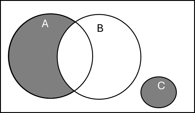
• 1. \(P(A \cup B) - P(B) + P(C)\)

• 2. \(P(A) - P(A \cap B) + P(C)\)

• 3. \(P(A) - P(B) + P(C)\)

• 4. \(P(A \cup C) - P(A \cap B)\)

• 5. \(P(A \cup B \cup C) - P(B)\)

Solution

Answer: (C)

The shaded region is \((A \setminus B) \cup C\), i.e., the part of \(A\) that does not intersect \(B\), together with all of \(C\). Its probability is \(P(A) - P(A \cap B) + P(C)\).

• (A) \(P(A \cup B) - P(B) + P(C) = P(A) - P(A \cap B) + P(C)\) — TRUE (by the inclusion-exclusion identity \(P(A \cup B) = P(A) + P(B) - P(A \cap B)\), so \(P(A \cup B) - P(B) = P(A) - P(A \cap B)\)).

• (B) \(P(A) - P(A \cap B) + P(C)\) — TRUE (directly matches the shaded region).

• (C) \(P(A) - P(B) + P(C)\) — FALSE. This subtracts all of \(P(B)\) rather than only the overlap \(P(A \cap B)\). It would give the wrong value whenever \(B\) extends outside \(A\).

• (D) \(P(A \cup C) - P(A \cap B)\) — TRUE (since \(A\) and \(C\) are disjoint, \(P(A \cup C) = P(A) + P(C)\)).

• (E) \(P(A \cup B \cup C) - P(B)\) — TRUE (since \(B\) is entirely inside \(A \cup B \cup C\), this correctly removes \(B\)’s contribution while retaining \(A \setminus B\) and \(C\)).

Therefore (C) is the expression that does NOT correctly represent the shaded probability.

Question 2.2 (3 pts)

Fréchet distribution is a heavily skewed, right-tailed continuous distribution that is used for modeling extreme events such as earthquake magnitudes, daily rainfall totals, and large insurance claims. Which of the following statements is TRUE about Fréchet distribution?

• 1. The mean is the largest among the measures of central tendency, followed by the mode and the median.

• 2. A small sample size is adequate to apply the central limit theorem to the distribution of the sample mean.

• 3. For samples from this distribution, the median and variance are recommended measures of central tendency and spread, respectively.

• 4. The interquartile range (IQR) is preferred for describing the spread of a population with a Fréchet distribution because it is less sensitive to outliers.

• 5. None of the above statements are TRUE for the Fréchet distribution.

Solution

Answer: (D)

• (A) FALSE. For a right-skewed distribution the correct ordering is mode < median < mean. Option (A) states the mean is the largest (correct), but then claims it is “followed by the mode and the median” — implying mean > mode > median. This reverses the relative positions of the mode and median; the correct descending order is mean > median > mode.

• (B) FALSE. The Fréchet distribution is heavily skewed with very heavy tails. A large sample size is required before the CLT provides a good normal approximation to \(\bar{X}\).

• (C) FALSE. The median is a good resistant measure of center, but the variance is not resistant to outliers. For a heavily skewed distribution the IQR is the preferred spread measure, not the variance.

• (D) TRUE. Because the Fréchet distribution is right-skewed with potential extreme values, the IQR is preferred over the standard deviation or variance as a measure of spread; it is not influenced by extreme observations in either tail.

• (E) FALSE, since (D) is true.

Question 2.3 (3 pts)

Suppose \(X\) is a random variable with \(E[2^X] = 16\), \(\text{Var}(X) = 32\), and \(E[3X + 2] = 8\). Let a new random variable \(Y\) be defined as \(Y = 2^X - \frac{1}{4}X^2\). What is \(E[Y]\)?

• 1. 0

• 2. 7

• 3. 8

• 4. 36

• 5. None of the above

Solution

Answer: (B) 7

Step 1: Find E[X] from \(E[3X + 2] = 8\).

\[3E[X] + 2 = 8 \implies E[X] = 2\]

Step 2: Find E[X²] using the variance formula.

\[\text{Var}(X) = E[X^2] - (E[X])^2 \implies 32 = E[X^2] - 4 \implies E[X^2] = 36\]

Step 3: Compute E[Y] using linearity of expectation.

\[E[Y] = E\!\left[2^X - \tfrac{1}{4}X^2\right] = E[2^X] - \tfrac{1}{4}E[X^2] = 16 - \tfrac{1}{4}(36) = 16 - 9 = \boxed{7}\]

Question 2.4 (3 pts)

An ANOVA F-test was performed on a dataset with two treatment levels (\(k = 2\)), resulting in a test statistic of \(F_{\text{TS}} = 3.28\). If the same dataset is used for a hypothesis test on the difference of means of the two levels, then \(t_{\text{TS}}^2 = 3.28\) only if:

• 1. The null value, \(\Delta_0\), is 0.

• 2. The hypothesis test is a two-tailed \(t\)-test.

• 3. The observations within and across the two levels are assumed to be independent.

• 4. The population variances are assumed to be equal, and the pooled variance estimate is used to construct the test statistic.

• 5. All of the above must hold simultaneously.

• 6. We cannot be certain because the \(F_{\text{TS}}\) and \(T_{\text{TS}}\) are test statistics for two different hypothesis tests, each with distinct assumptions and interpretations.

Solution

Answer: (E)

The algebraic identity \(F_{\text{TS}} = t_{\text{TS}}^2\) holds between the one-way ANOVA F-test (with \(k = 2\)) and the two-sample \(t\)-test only when all four conditions are simultaneously satisfied:

• (A) The null value must be \(\Delta_0 = 0\), so the ANOVA null (\(\mu_1 = \mu_2\)) aligns with the \(t\)-test null (\(\mu_1 - \mu_2 = 0\)).

• (B) The \(t\)-test must be two-tailed, because squaring the test statistic loses directional information and corresponds to the upper-tail F rejection region.

• (C) Independence within and across groups must be assumed by both tests.

• (D) The pooled variance estimate must be used in the \(t\)-test; the ANOVA MSE is exactly the pooled variance estimate \(s_p^2\).

If any condition fails — for example, if the \(t\)-test uses Welch’s (unpooled) variance or is one-sided — then \(t_{\text{TS}}^2 \neq F_{\text{TS}}\). Hence all conditions must hold simultaneously.

Question 2.5 (3 pts)

Which of the following statements is true for simple linear regression?

• 1. All diagnostics plots rely on the residuals/errors.

• 2. The assumption that the response is a simple random sample (SRS) for each fixed value of the explanatory variable is easy to verify.

• 3. A scatter plot can be used to assess both linearity and normality.

• 4. A scatter plot can be used to assess both homogeneity of variance and linearity.

• 5. All of the above are true for simple linear regression.

Solution

Answer: (D)

• (A) FALSE. The scatter plot of \(Y\) vs. \(x\) is a diagnostic plot that does not rely on residuals; it is used to assess linearity directly from raw data.

• (B) FALSE. The independence/SRS assumption cannot be verified from the data alone; it depends on the study design and data collection procedure.

• (C) FALSE. A scatter plot can be used to assess linearity, but not normality of errors. Normality is assessed using a histogram or QQ-plot of the residuals.

• (D) TRUE. A scatter plot can reveal whether the spread of \(Y\) values around the apparent trend changes as \(x\) changes (homogeneity of variance) and whether the trend itself appears linear.

—

Problem 3 Setup

A dietitian is studying the effectiveness of a new dietary supplement on weight loss. To evaluate its impact, the dietitian measures the weight of 44 individuals before and after a 4-week regimen with the supplement.

The difference in weight (\(d\) = weight after − weight before) is calculated for each participant. The dietitian wants to establish whether the supplement results in a decrease in weight. The dietitian would like the test to have at least 90% power to detect an average weight decrease of 6 lbs, which is deemed an important reduction.

The test is conducted at a significance level of \(\alpha = 0.05\), with hypotheses:

\[H_0\colon \mu_d \geq 0 \qquad H_a\colon \mu_d < 0\]

For this paired test, the standard deviation of the differences, \(\sigma_d\), is assumed to be known with a value of 12 lbs.

Problem 3 — Power Analysis (16 points)

Question 3a (3 pts)

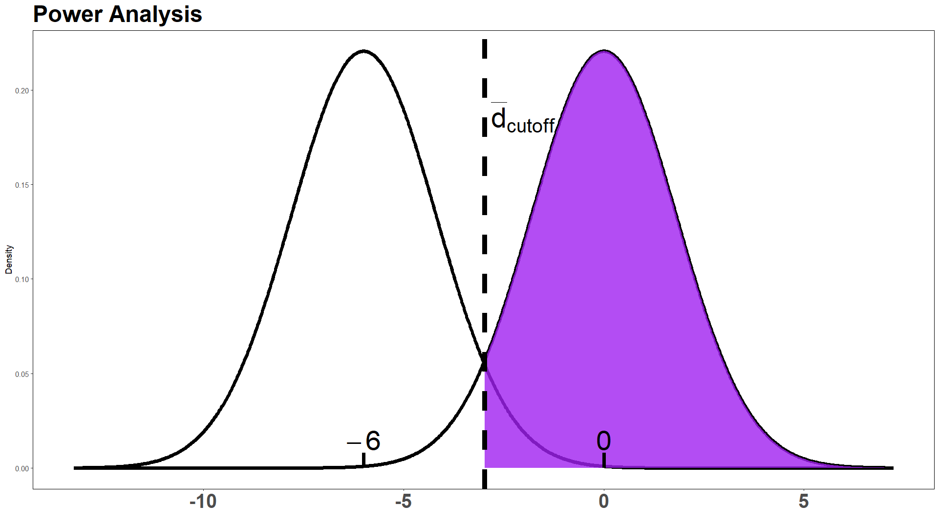
Select the correct option for what the purple shaded region in the power graph actually represents.

• 1. The intern is correct; it is the power of the test in detecting an alternative \(\mu_{d_a} = -6\).

• 2. The intern is wrong; it is in fact the probability of Type I error.

• 3. The intern is wrong; it is in fact the probability of Type II error.

• 4. The intern is wrong, and it is none of the above options.

Solution

Answer: (D)

The graph shows two normal curves: one centered at \(\mu_d = -6\) (the alternative distribution) and one centered at \(\mu_d = 0\) (the null distribution). The vertical dashed line marks \(\bar{d}_{\text{cutoff}}\).

The purple region is the area to the right of \(\bar{d}_{\text{cutoff}}\) under the null distribution (centered at 0). Since the rejection region for this left-tailed test is \(\bar{D} < \bar{d}_{\text{cutoff}}\), the purple region is the non-rejection region under the null distribution, which has area \(1 - \alpha = 0.95\).

• Power = area to the left of \(\bar{d}_{\text{cutoff}}\) under the alternative distribution — this is not what is shaded (wrong distribution, wrong tail).

• Type I error (\(\alpha\)) = area to the left of \(\bar{d}_{\text{cutoff}}\) under the null distribution — this is not what is shaded (wrong tail).

• Type II error (\(\beta\)) = area to the right of \(\bar{d}_{\text{cutoff}}\) under the alternative distribution — this is not what is shaded (wrong distribution).

The purple region corresponds to none of these, so the intern is wrong and the answer is (D).

Question 3b (13 pts)

Using the R output below, calculate the power of the test to detect an average weight decrease of 6 lbs. Determine whether the sample size is sufficient to meet the dietitian’s requirement for at least 90% power. Provide a detailed explanation of your calculations, including all steps and reasoning, to receive full credit. This includes computing \(\bar{d}_{\text{cutoff}}\) and writing out full probability statements.

> qnorm(p = 0.05, lower.tail = FALSE)
[1] 1.644854
> qt(p = 0.05, df = 43, lower.tail = FALSE)
[1] 1.681071
> qnorm(p = 0.1, lower.tail = FALSE)
[1] 1.281552
> qt(p = 0.1, df = 43, lower.tail = FALSE)
[1] 1.301552
> pnorm(1.671771, lower.tail = TRUE)
[1] 0.9527153
> pnorm(1.671771, lower.tail = FALSE)
[1] 0.04728474
> pnorm(-2.975653, lower.tail = TRUE)
[1] 0.001461827
> pnorm(-2.975653, lower.tail = FALSE)
[1] 0.9985382
> pt(1.671771, df = 43, lower.tail = TRUE)
[1] 0.9490839
> pt(1.671771, df = 43, lower.tail = FALSE)
[1] 0.05091613
> pt(-2.975653, df = 43, lower.tail = TRUE)
[1] 0.002391402
> pt(-2.975653, df = 43, lower.tail = FALSE)
[1] 0.9976086

Solution

Answer: Power = 0.9527; yes, the sample size is sufficient.

Since \(\sigma_d = 12\) is known, we use the z-test framework.

Step 1 — Select the critical value.

For a left-tailed test at \(\alpha = 0.05\) with known \(\sigma\):

> qnorm(p = 0.05, lower.tail = FALSE)
[1] 1.644854

We use \(z_{0.05} = 1.644854\).

Step 2 — Compute :math:`bar{d}_{text{cutoff}}`.

The rejection region is \(\bar{D} < \bar{d}_{\text{cutoff}}\), where:

\[P\!\left(\bar{D} < \bar{d}_{\text{cutoff}} \mid \mu_d = 0\right) = 0.05\]

Solving:

\[\bar{d}_{\text{cutoff}} = \mu_0 - z_{0.05} \cdot \frac{\sigma_d}{\sqrt{n}} = 0 - 1.644854 \times \frac{12}{\sqrt{44}} = -2.9757\]

Step 3 — Set up the power probability statement.

The power at \(\mu_{d_a} = -6\) is:

\[\text{Power} = P\!\left(\bar{D} < \bar{d}_{\text{cutoff}} \mid \mu_d = -6\right) = P\!\left(Z < \frac{\bar{d}_{\text{cutoff}} - (-6)}{\sigma_d/\sqrt{n}}\right)\]

\[= P\!\left(Z < \frac{-2.9757 + 6}{12/\sqrt{44}}\right) = P(Z < 1.671771)\]

Step 4 — Read the power from the R output.

> pnorm(1.671771, lower.tail = TRUE)
[1] 0.9527153

\[\text{Power} = \boxed{0.9527}\]

Conclusion: Since \(0.9527 > 0.90\), the sample size of \(n = 44\) is sufficient to achieve the dietitian’s requirement of at least 90% power.

—

Problem 4 Setup

Halin is a new student in STAT 350 and has never coded in R before. To improve her skills, she spends at most 40 minutes each weekday doing R self-study. Her daily workflow is as follows:

• The time it takes until she runs into an error, denoted by \(T\), follows an Exponential distribution with an average time of 25 minutes.

• If \(T > 40\), she does not run into an error during her study session that day.

• If \(T \leq 40\), she encounters an error and attempts to debug it:

  • Debugging succeeds with probability 0.7, after which she feels happy and ends her study session.

  • Debugging fails with probability 0.3, and she immediately stops and goes to office hours for help.

• Each day’s workflow is independent of other days.

Problem 4 — Exponential Distribution and Binomial (30 points)

Question 4a (8 pts)

What is the probability that Halin will complete her study session on a given weekday without encountering an error?

Solution

Answer: 0.2019

Since \(T \sim \text{Exponential}\!\left(\lambda = \frac{1}{25}\right)\) (rate = 1/25, mean = 25):

\[P(T > 40) = e^{-\lambda \cdot 40} = e^{-40/25} = e^{-1.6} \approx \boxed{0.2019}\]

Question 4b (12 pts)

On a given weekday, what is the probability that Halin does not need to go to office hours?

Solution

Answer: 0.7606 (exact: 0.760569)

Halin avoids office hours in two mutually exclusive scenarios: (1) she finishes without an error (\(T > 40\)), or (2) she encounters an error but debugging succeeds (\(T \leq 40\) and debug success). Because these two events are mutually exclusive, the addition rule applies; expanding the second event by the multiplication rule gives:

\[P(\text{No Office Hours}) = P(T > 40) + P(\text{Debug Success} \mid T \leq 40) \cdot P(T \leq 40)\]

\[= e^{-1.6} + 0.7 \times (1 - e^{-1.6})\]

\[= 0.2019 + 0.7 \times 0.7981 = 0.2019 + 0.5587 = \boxed{0.7606}\]

(Exact, without intermediate rounding: \(0.760569\).)

Question 4c (10 pts)

Suppose Halin has continued her independent study for 20 weekdays. Use the information from the previous question to determine the probability that Halin will visit office hours exactly 5 times over the 20 weekdays.

Solution

Answer: 0.2011

Let \(N\) = number of office hours visits over 20 independent weekdays. Since each day is independent with:

\[p = P(\text{Office Hours}) = 1 - 0.760569 = 0.239431\]

we have \(N \sim \text{Binomial}(n = 20,\ p = 0.239431)\).

\[P(N = 5) = \binom{20}{5} \times (0.239431)^5 \times (0.760569)^{15} = \boxed{0.2011}\]

Note on key rounding ⚠️

The solution key presents a “rounded” version using \(p = 1 - 0.7657 = 0.2343\), yielding \(P(N=5) = 0.1996\). However, rounding \(P(\text{No OH}) = 0.760569\) to four decimal places gives \(0.7606\), not \(0.7657\). The value \(0.7657\) appears to be a transcription error in the key. The correct four-decimal-rounded probability is \(p = 1 - 0.7606 = 0.2394\), which gives \(P(N=5) \approx 0.2011\) — consistent with the unrounded calculation. The key’s own “exact” answer of \(0.201106\) confirms this.

—

Problem 5 Setup

A clothing retail company aims to boost profit during the upcoming holiday season, and its marketing team has decided to use four advertising strategies: an Email Ad Campaign, a Direct Mail Ad Campaign, a Social Media Ad Campaign, and an AI-Powered Ad Campaign. To test the effectiveness of these strategies, 180 loyal customers were randomly divided into four groups of 45 customers each. Each group was exposed to one advertising strategy, and their purchase amounts for the year were recorded.

Table 15 Summary Statistics by Ad Campaign

	Email	Direct Mail	Social Media	AI-Powered
\(n_i\)	45	45	45	45
\(\bar{x}_i\)	449.45	450.39	453.42	455.72
\(s_i^2\)	68.16	104.6542	112.3643	147.7942

Problem 5 — One-Way ANOVA (42 points)

Question 5a (3 pts)

Which of the following assumptions is NOT required to perform one-way ANOVA? Assume a factor has \(k\) levels.

• 1. Population variances are equal across the \(k\) groups.

• 2. An independent sample is randomly drawn from each of the \(k\) groups.

• 3. Observations within each group are independent of observations in other groups.

• 4. The sample sizes from each of the \(k\) groups are the same.

• 5. The sample means are normally distributed for each of the \(k\) groups.

• 6. All of the above assumptions are required.

Solution

Answer: (D)

One-way ANOVA requires: (A) equal variances (homogeneity of variance), (B) independent random samples from each group, (C) independence within and across groups, and (E) normality of observations within each group (which, by the CLT, implies the sample means are approximately normal). However, equal sample sizes are not required. ANOVA can be performed with unbalanced designs (different \(n_i\)). Therefore (D) is the assumption that is NOT required.

Question 5b (2 pts)

Determine whether the homogeneity of variance assumption is valid or invalid. Mathematically support your answer.

Solution

Answer: The equal variance assumption holds (VALID).

The rule of thumb checks whether the ratio of the largest to smallest sample standard deviation is at most 2:

\[\frac{s_{\max}}{s_{\min}} = \frac{\sqrt{147.7942}}{\sqrt{68.16}} = \frac{12.1572}{8.2561} \approx 1.473 \leq 2\]

Since the ratio is less than 2, the homogeneity of variance assumption is satisfied.

Question 5c (4 pts)

Clearly identify the factor of interest, specify how many levels this factor has, and describe what the quantitative response variable measures. Using this information, define the parameters of interest and state the null hypothesis and alternative hypothesis.

Solution

Factor of interest: Type of Ad Campaign — with 4 levels (Email, Direct Mail, Social Media, AI-Powered).

Response variable: Purchase amount for the year (in dollars) — a quantitative measure of how much a customer spent.

Parameters of interest: Let \(\mu_{\text{Email}}\), \(\mu_{\text{Direct}}\), \(\mu_{\text{Social}}\), \(\mu_{\text{AI}}\) denote the true mean yearly purchase amounts for customers exposed to each of the four ad campaign types, respectively.

\[H_0\colon \mu_{\text{Email}} = \mu_{\text{Direct}} = \mu_{\text{Social}} = \mu_{\text{AI}}\]

\[H_a\colon \mu_i \neq \mu_j \text{ for some } i \neq j\]

In words: \(H_0\) states that the true mean yearly purchase amount is the same across all four advertising strategies. \(H_a\) states that at least two of the strategies produce different mean yearly purchase amounts.

Question 5d (12 pts)

Complete the ANOVA table. Clearly show your work.

Table 16 One-Way ANOVA Table

Source	df	SS	MS	F
Factor (Ad Campaign)	3	1111.9185	370.6395	3.4241
Error	176	19050.80	108.2432
Total	179	20162.72

Solution

Work shown below.

Degrees of freedom:

\[\text{df}_A = k - 1 = 4 - 1 = 3\]

\[\text{df}_E = N - k = 180 - 4 = 176\]

\[\text{df}_T = N - 1 = 179\]

SSE (using pooled within-group variance):

\[\text{SSE} = \sum_{i=1}^{4}(n_i - 1)s_i^2 = 44(68.16 + 104.6542 + 112.3643 + 147.7942) = 44 \times 432.9727 = 19050.80\]

MSE:

\[\text{MSE} = \frac{\text{SSE}}{\text{df}_E} = \frac{19050.80}{176} = 108.2432\]

SSA (using overall mean \(\bar{\bar{x}} = (449.45 + 450.39 + 453.42 + 455.72)/4 = 452.245\)):

\[\text{SSA} = \sum_{i=1}^{4} n_i(\bar{x}_i - \bar{\bar{x}})^2 = 45\left[(449.45 - 452.245)^2 + (450.39 - 452.245)^2 + (453.42 - 452.245)^2 + (455.72 - 452.245)^2\right]\]

\[= 45[(-2.795)^2 + (-1.855)^2 + (1.175)^2 + (3.475)^2]\]

\[= 45[7.8120 + 3.4410 + 1.3806 + 12.0756] = 45 \times 24.7093 = 1111.92\]

MSA:

\[\text{MSA} = \frac{\text{SSA}}{\text{df}_A} = \frac{1111.92}{3} = 370.6395\]

F-statistic:

\[F_{\text{TS}} = \frac{\text{MSA}}{\text{MSE}} = \frac{370.6395}{108.2432} = 3.4241\]

SST = SSA + SSE = 1111.92 + 19050.80 = 20162.72.

Question 5e (7 pts)

The \(p\)-value was found to be 0.0185. Test your hypotheses at a significance level of \(\alpha = 0.05\). Provide the formal decision and interpret the conclusion in the context of the problem. You may assume all assumptions are valid.

Solution

Decision: Reject \(H_0\).

Since \(p\text{-value} = 0.0185 < 0.05 = \alpha\), we reject \(H_0\).

The data give support (\(p\)-value \(= 0.0185\)) to the claim that there is a difference in the true mean yearly purchase amount among customers exposed to at least two of the four advertising strategies. At the 5% significance level, we conclude that not all four ad campaigns produce the same average yearly spending.

Question 5f (3 pts)

Based on your conclusion, determine whether you should proceed to conduct a Tukey HSD test.

• 1. Conduct the Tukey HSD test because it can identify specific pairs of means that are significantly different when the ANOVA results show a significant difference.

• 2. Do not conduct the Tukey HSD test because the ANOVA results indicate that the population means are not significantly different.

• 3. There is insufficient information provided to decide whether a Tukey HSD test should be conducted.

Solution

Answer: (A)

Because the ANOVA F-test rejected \(H_0\), we know that at least one pair of group means differs, but we do not know which pairs differ. The Tukey HSD test is a post-hoc multiple comparisons procedure that controls the family-wise error rate while identifying which specific pairs are significantly different. We proceed with the Tukey HSD test.

Question 5g (3 pts)

Regardless of your conclusion for part (f), the researchers decided to conduct a Tukey HSD with an overall significance level of 5%. Let \(\text{df}_E\) denote the correct degrees of freedom for error. Choose the correct Tukey parameter.

• 1. qtukey(0.95, nmeans = 3, df = dfe, lower.tail=TRUE) = 3.342793

• 2. qtukey(0.95/2, nmeans = 4, df = dfe, lower.tail=TRUE) = 1.925889

• 3. qtukey(0.95/2, nmeans = 3, df = dfe, lower.tail=TRUE) = 1.533567

• 4. qtukey(0.95, nmeans = 4, df = dfe, lower.tail=TRUE) = 3.66811

Solution

Answer: (D)

The Tukey HSD procedure requires qtukey(1 - α, nmeans = k, df = df_E). Here:

• \(\alpha = 0.05\), so we use 1 - α = 0.95.

• \(k = 4\) groups (nmeans = 4).

• \(\text{df}_E = 176\).

Options (A) and (C) use nmeans = 3 (incorrect — there are 4 groups). Options (B) and (C) use 0.95/2 (incorrect — the Tukey quantile is not halved). Only (D) has both the correct confidence level (0.95) and the correct number of means (4).

Question 5h (8 pts)

Using the summary information and the Tukey parameter above, construct a 95% confidence interval for the true difference in the average yearly amount spent by customers exposed to the AI-powered Ad Campaign and those exposed to the Direct Mail Ad Campaign. Based on the confidence interval, determine whether there is statistically significant evidence of a difference between these two groups.

Solution

Answer: (−0.3590, 11.0190); no statistically significant difference.

Given: \(\bar{x}_{\text{AI}} = 455.72\), \(\bar{x}_{\text{Direct}} = 450.39\), \(\text{MSE} = 108.2432\), \(n_{\text{AI}} = n_{\text{Direct}} = 45\), \(q = 3.66811\).

The Tukey 95% CI for \(\mu_{\text{AI}} - \mu_{\text{Direct}}\) is:

\[\left(\bar{x}_{\text{AI}} - \bar{x}_{\text{Direct}}\right) \pm \frac{q}{\sqrt{2}}\sqrt{\text{MSE}\left(\frac{1}{n_{\text{AI}}} + \frac{1}{n_{\text{Direct}}}\right)}\]

\[= (455.72 - 450.39) \pm \frac{3.66811}{\sqrt{2}}\sqrt{108.2432 \times \frac{2}{45}}\]

\[= 5.33 \pm 2.5937\sqrt{4.8108}\]

\[= 5.33 \pm 2.5937 \times 2.1934\]

\[= 5.33 \pm 5.6900\]

\[\boxed{(-0.3590,\ 11.0190)}\]

Since the interval contains 0, there is no statistically significant evidence at the 5% family-wise error level that the true mean yearly spending differs between customers exposed to the AI-powered campaign and those exposed to the Direct Mail campaign.

—

Problem 6 Setup

A STAT 350 student sought to explore the relationship between the cost of a meal for a single diner (\(x\)) and the tip amount offered (\(Y\)). The student selected nine specific meal costs and, for each cost, recorded a randomly selected tip amount from diners at a restaurant in Greater Lafayette.

Table 17 Meal Cost and Tip Data

Variable	1	2	3	4	5	6	7	8	9
Meal cost (\(x\), $)	33.85	31.24	26.82	38.54	33.97	36.44	30.13	29.65	32.76
Tip (\(Y\), $)	5.35	6.48	7.52	3.63	4.75	4.23	5.87	6.55	4.86

Problem 6 — Simple Linear Regression (44 points)

Question 6a (5 pts)

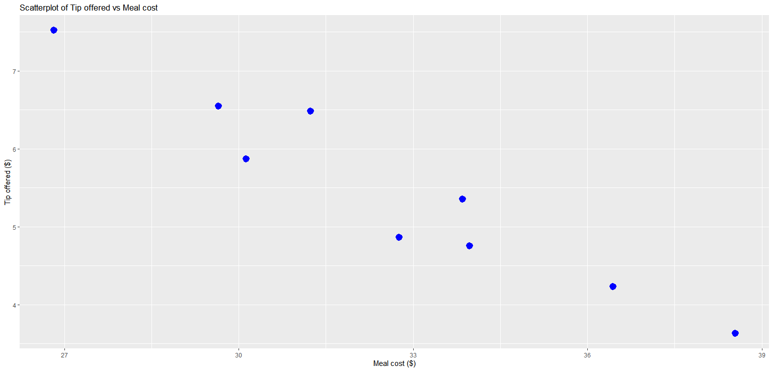
Describe the relationship between meal cost and the tip amount based on the scatter plot below.

Solution

Answer: The relationship between meal cost and tip amount is linear with a negative direction and a strong to moderate association. As meal cost increases, the tip amount tends to decrease.

Question 6b (15 pts)

The following summary statistics were realized from the data above:

\[n = 9, \quad \bar{x} = 32.600, \quad \bar{y} = 5.4711\]

\[\sum_{i=1}^{9} x_i y_i = 1570.9020, \quad \sum_{i=1}^{9} x_i^2 = 9668.3960, \quad \sum_{i=1}^{9} y_i^2 = 281.7746\]

1. Determine the slope (\(b_1\)) of the least-squares regression line.

2. Determine the intercept (\(b_0\)) of the least-squares regression line.

3. Write out the equation of the regression line.

Solution

(i) Slope:

\[S_{xy} = \sum x_i y_i - n\bar{x}\bar{y} = 1570.9020 - 9 \times 32.600 \times 5.4711 = 1570.9020 - 1605.2238 = -34.3218\]

\[S_{xx} = \sum x_i^2 - n\bar{x}^2 = 9668.3960 - 9 \times (32.600)^2 = 9668.3960 - 9564.84 = 103.556\]

\[b_1 = \frac{S_{xy}}{S_{xx}} = \frac{-34.3218}{103.556} = \boxed{-0.3314}\]

(ii) Intercept:

\[b_0 = \bar{y} - b_1 \bar{x} = 5.4711 - (-0.3314335)(32.600) = 5.4711 + 10.8047 = \boxed{16.2758}\]

(iii) Regression equation:

\[\hat{y} = 16.2758 - 0.3314 \, x_{\text{Meal Cost}}\]

Interpretation of slope: For each additional dollar in meal cost, the estimated tip amount decreases by approximately $0.33.

Question 6c (6 pts)

List the assumptions of simple linear regression that can be evaluated using diagnostic plots. For each assumption, specify all the diagnostic plots that can be used to assess it. To receive full credit, you must include all relevant plots for each assumption.

Solution

Three of the four LINE assumptions can be assessed graphically:

Linearity: The relationship between \(x\) and \(Y\) is linear.

• Diagnostic plots: Scatter plot (of \(Y\) vs. \(x\)) and Residual plot (of residuals \(e_i\) vs. fitted values \(\hat{y}_i\)). A non-linear pattern in either plot indicates a violation.

Homogeneity of variance (Equal variance): The variance of the errors \(\epsilon_i\) is constant for all values of \(x\).

• Diagnostic plots: Scatter plot and Residual plot. Fanning or systematic changes in spread across the plot indicate heteroscedasticity.

Normality of errors: The errors \(\epsilon_i\) are normally distributed.

• Diagnostic plots: Histogram of residuals (should be approximately bell-shaped) and Normal QQ-plot of residuals (points should follow the reference line).

Note

The Independence assumption (errors are independent) cannot be assessed from standard diagnostic plots; it depends on the study design and data collection.

Question 6d (18 pts)

The following output was obtained using RStudio for the tip–meal cost data. You may assume that all assumptions have been met for simple linear regression.

Residual standard error: 0.3783 on 7 degrees of freedom
Multiple R-squared:  0.9191,    Adjusted R-squared:  0.9075
F-statistic: 79.49 on 1 and 7 DF,  p-value: 4.534e-05

1. Interpret the coefficient of determination, \(R^2\), given in the output above.

2. Use the output above and your results in (b) to compute the Pearson correlation coefficient (\(r\)).

3. For the test on the slope \(\beta_1\): use the output above to calculate the \(t\)-test statistic, and specify the associated degrees of freedom.

4. Perform a four-step hypothesis test at \(\alpha = 0.01\) using the F-test procedure to determine whether there is a significant linear association between meal cost and tip offered.

Solution

(i) Interpretation of R²:

\(R^2 = 0.9191\). Approximately 91.91% of the variation in tip amount is explained by the linear relationship with meal cost. This indicates a very strong linear fit.

(ii) Pearson correlation coefficient:

Since \(b_1 = -0.3314 < 0\), the association is negative, so:

\[r = -\sqrt{R^2} = -\sqrt{0.9191} \approx \boxed{-0.9587}\]

(iii) t-test statistic for \(\beta_1\):

For simple linear regression, \(F_{\text{TS}} = t_{\text{TS}}^2\). Since \(b_1 < 0\):

\[t_{\text{TS}} = -\sqrt{F_{\text{TS}}} = -\sqrt{79.49} \approx \boxed{-8.9157}\]

Degrees of freedom: \(\text{df}_E = n - 2 = 9 - 2 = 7\).

(iv) Four-step F-test:

Step 1 — Parameter of interest: Let \(\beta_1\) represent the true slope of the linear relationship between meal cost (\(x\)) and tip amount (\(Y\)) at the restaurant.

Step 2 — Hypotheses:

\[H_0\colon \beta_1 = 0 \quad \text{(no linear association between meal cost and tip amount)}\]

\[H_a\colon \beta_1 \neq 0 \quad \text{(there is a linear association between meal cost and tip amount)}\]

Step 3 — Test statistic and p-value:

From the R output:

\[F_{\text{TS}} = 79.49, \quad \text{df}_M = 1, \quad \text{df}_E = 7, \quad p\text{-value} = 4.534 \times 10^{-5}\]

Step 4 — Decision and conclusion:

Since \(p\text{-value} = 4.534 \times 10^{-5} < 0.01 = \alpha\), we reject \(H_0\).

The data give support (\(p\)-value \(= 4.534 \times 10^{-5}\)) to the claim that there is a significant linear association between the cost of a meal and the tip amount offered at the restaurant in Greater Lafayette.