Slides 📊

Download Chapter 6 slides (PPTX)

6.2. Expected Value and Variance of Continuous Random Variables

Now that we understand how probability density functions work for continuous random variables, we need to extend our concepts of expected value and variance from the discrete world. The core ideas remain the same—we still want to measure the center and spread of a distribution—but the mathematical machinery shifts from summation to integration. This transition reveals the beautiful parallel structure between discrete and continuous probability theory.

Road Map 🧭

• Extend expected value from discrete sums to continuous integrals.

• Apply the Law of the Unconscious Statistician (LOTUS) for functions of continuous random variables.

• Understand that the linearity and additive properties of expected values remain unchanged.

• Define variance using integration and master the computational shortcut.

• Explore properties of variance for linear transformations and sums of independent variables.

6.2.1. From Discrete Sums to Continuous Integrals

The expected value of a discrete random variable involved summing each possible value, weighted by its probability. For continuous random variables, we replace this discrete sum with a continuous integral, weighing each possible value by its probability density.

Definition

The expected value of a continuous random variable \(X\), denoted \(E[X]\) or \(\mu_X\), is the continuously weighted average of all values in its support:

\[\mu_X = E[X] = \int_{-\infty}^{\infty} x \cdot f_X(x) \, dx\]

This integral represents the “balance point” or center of mass of the probability distribution. Just as in the discrete case, values with higher probability density contribute more to the overall average.

Comparison with the Discrete Case

Discrete \(E[X]\)	Continuous \(E[X]\)
\[\sum_{x \in \text{supp}(X)} x \cdot p_X(x)\]	\[\int_{-\infty}^{\infty} x \cdot f_X(x) \, dx = \int_{\text{supp}(X)}x \cdot f_X(x) \, dx\]

The summation becomes an integration, and the probability mass function \(p_X(x)\) is replaced by the probability density function \(f_X(x)\). Although the integral is formally taken over the entire real line \((-\infty, \infty)\) in the general definition of continuous expectation, only values of \(x\) within the support contribute meaningfully to the computation, since \(f_X(x) = 0\) outside \(\text{supp}(X)\). Thus, the integral is effectively taken over the support—just as the summation is in the discrete case.

Remark: The Absolute Integrability Condition

For the expected value of \(X\) to be well-defined and finite, \(X\) must satisfy

\[\int_{-\infty}^{\infty} |x| \cdot f_X(x) \, dx < \infty.\]

All continuous distributions we encounter in this course satisfy this condition.

6.2.2. The Law of the Unconscious Statistician (LOTUS) for Continuous Random Variables

Just as in the discrete case, we often want to find the expected value of some function of a random variable, like \(E[X^2]\) or \(E[e^X]\). The Law of the Unconscious Statistician (LOTUS) extends naturally to continuous random variables.

Theorem: LOTUS

If \(X\) is a continuous random variable with PDF \(f_X(x)\), and \(g(x)\) is a function, then:

\[E[g(X)] = \int_{-\infty}^{\infty} g(x) \cdot f_X(x) \, dx\]

The Power of LOTUS

This theorem is powerful because it allows us to compute \(E[g(X)]\) directly without having to find the PDF of the new random variable \(Y = g(X)\). Instead, we simply plug \(g(x)\) into our expectation integral and use the original PDF \(f_X(x)\).

Example💡: Expected value of functions of \(X\)

Consider a continuous random variable \(X\) with PDF

\[\begin{split}f_X(x) = \begin{cases} &2x, &0 \leq x \leq 1\\ &0, & \text{ elsewhere } \end{cases}.\end{split}\]

Find \(E[X], E[X^2]\), and \(E[\sqrt{X}]\).

• Find \(E[X]\) using the definition

  \[E[X] = \int_0^1 x \cdot (2x) \, dx = \int_0^1 2x^2 \, dx = 2 \cdot \frac{x^3}{3}\Bigg\rvert_0^1 = \frac{2}{3}\]

• Apply LOTUS for \(E[X^2]\) and \(E[\sqrt{X}]\)

\[E[X^2] = \int_0^1 x^2 \cdot (2x) \, dx = \int_0^1 2x^3 \, dx = 2 \cdot \frac{x^4}{4}\Bigg\rvert_0^1 = \frac{1}{2}\]

\[E[\sqrt{X}] = \int_0^1 x^{1/2} \cdot 2x \, dx = \int_0^1 2x^{3/2} \, dx = 2\cdot \frac{2}{5}x^{5/2}\Bigg\rvert_{0}^1 = \frac{4}{5}\]

6.2.3. Properties of Expected Value: Unchanged by Continuity

The fundamental properties of expected value that we learned for discrete random variables apply unchanged to continuous random variables.

Linearity of Expectation

For any continuous random variable \(X\) and constants \(a\) and \(b\):

\[E[aX + b] = aE[X] + b\]

Proof of linearity of expectation

\[\begin{split}\begin{aligned} E[aX + b] &= \int_{-\infty}^{\infty} (ax + b) \cdot f_X(x) \, dx \\ &= a\int_{-\infty}^{\infty} x \cdot f_X(x) \, dx + b\int_{-\infty}^{\infty} f_X(x) \, dx \\ &= aE[X] + b \cdot 1 \\ &= aE[X] + b \end{aligned}\end{split}\]

Additivity of Expectation

For any set of continuous random variables \(X_1, X_2, \cdots, X_n\),

\[E[X_1 + X_2 + \cdots + X_n] = E[X_1] + E[X_2] + \cdots + E[X_n]\]

6.2.4. Variance for Continuous Random Variables

Definition

The variance of a continuous random variable \(X\) is the expected value of the squared deviation from the mean:

\[\sigma_X^2 = \text{Var}(X) = E[(X - \mu_X)^2] = \int_{-\infty}^{\infty} (x - \mu_X)^2 \cdot f_X(x) \, dx\]

Computational Shortcut for Variance

Just as in the discrete case, we have the much more convenient computational formula:

\[\sigma_X^2 = E[X^2] - (E[X])^2\]

Standard Deviation

The standard deviation is the square root of the variance:

\[\sigma_X = \sqrt{\text{Var}(X)}\]

Example💡: Computing Variance

For the random variable \(X\) with PDF

\[\begin{split}f_X(x) = \begin{cases} &2x, &0 \leq x \leq 1\\ &0, &\text{ elsewhere } \end{cases},\end{split}\]

compute \(\text{Var}(X)\) and \(\sigma_X\).

Using \(E[X]\) and \(E[X^2]\) obtained in the previous example, apply the computational shortcut:

\[\text{Var}(X) = E[X^2] - (E[X])^2 = \frac{1}{2} - \left(\frac{2}{3}\right)^2 = \frac{1}{2} - \frac{4}{9} = \frac{9-8}{18} = \frac{1}{18}\]

Therefore, \(\sigma_X = \sqrt{1/18} = 1/(3\sqrt{2}) \approx 0.236\).

6.2.5. Properties of Variance for Continuous Random Variables

The variance properties we learned for discrete random variables apply without modification to continuous random variables.

Variance of Linear Transformations

For any continuous random variable \(X\) and constants \(a\) and \(b\):

\[\text{Var}(aX + b) = a^2 \text{Var}(X)\]

Recall that:

• Adding a constant (\(b\)) doesn’t change how spread out a distribution is—it just shifts its location.

• Multiplying by a constant (\(a\)) scales the variance by \(a^2\).

Variance of Sums of Independent Random Variables

When \(X\) and \(Y\) are independent continuous random variables:

\[\text{Var}(X + Y) = \text{Var}(X) + \text{Var}(Y).\]

This extends to any number of mutually independent variables:

\[\text{Var}(X_1 + X_2 + \cdots + X_n) = \text{Var}(X_1) + \text{Var}(X_2) + \cdots + \text{Var}(X_n).\]

Be Cautious 🛑

The additivity of variances only applies when the random variables are independent. This means that the mutual independence of all terms involved must be provided or mathematically shown before the rule is applied.

For dependent variables, we need to account for covariance terms.

6.2.6. Covariance and Correlation: A Brief Introduction

When dealing with multiple continuous random variables that may be dependent, we need measures of how they vary together. The concepts of covariance and correlation also extend to continuous random variables.

Covariance

The covariance between continuous random variables \(X\) and \(Y\) is:

\[\text{Cov}(X,Y) = E[(X - \mu_X)(Y - \mu_Y)] = E[XY] - \mu_X\mu_Y\]

Correlation

The correlation coefficient is:

\[\rho_{X,Y} = \frac{\text{Cov}(X,Y)}{\sigma_X \sigma_Y}.\]

As before, correlation is unitless and bounded between -1 and +1.

Note

Working with continuous joint distributions involves multivariable calculus and is beyond the scope of this course. We’ll focus on single continuous random variables in the remainder of this chapter.

6.2.7. Bringing It All Together

Key Takeaways 📝

1. The expected value of a continuous random variable uses integration instead of summation, but represents the same concept: a weighted average using probability densities as weights.

2. All properties of expectation (LOTUS, linearity, additivity) remain unchanged—only the computational method (integration vs. summation) differs.

3. Variance maintains the same conceptual meaning and computational shortcut.

4. Variance properties for linear transformations and sums of independent variables apply identically to continuous random variables.

6.2.8. Exercises

These exercises develop your skills in computing expected values and variances for continuous random variables using integration, applying LOTUS for functions of random variables, and using the properties of expectation and variance.

---

Exercise 1: Basic Expected Value and Variance Computation

A biomedical engineer models the concentration \(X\) (in mg/L) of a drug in a patient’s bloodstream with the following PDF:

\[\begin{split}f_X(x) = \begin{cases} 3x^2, & 0 \leq x \leq 1\\ 0, & \text{elsewhere} \end{cases}\end{split}\]

1. Verify this is a valid PDF.

2. Find \(E[X]\), the expected drug concentration.

3. Find \(E[X^2]\) using LOTUS.

4. Calculate \(\text{Var}(X)\) using the computational shortcut.

5. Find the standard deviation \(\sigma_X\).

6. If the therapeutic range requires concentrations within one standard deviation of the mean, what is this range?

Solution

Part (a): Verify PDF validity

Non-negativity: \(3x^2 \geq 0\) for all \(x \in [0, 1]\). ✓

Total area = 1:

\[\int_0^1 3x^2 \, dx = 3 \cdot \frac{x^3}{3} \Bigg|_0^1 = x^3 \Bigg|_0^1 = 1 - 0 = 1 \text{ ✓}\]

Part (b): E[X]

\[E[X] = \int_0^1 x \cdot 3x^2 \, dx = 3\int_0^1 x^3 \, dx = 3 \cdot \frac{x^4}{4} \Bigg|_0^1 = \frac{3}{4} = 0.75 \text{ mg/L}\]

Part (c): E[X²] using LOTUS

\[E[X^2] = \int_0^1 x^2 \cdot 3x^2 \, dx = 3\int_0^1 x^4 \, dx = 3 \cdot \frac{x^5}{5} \Bigg|_0^1 = \frac{3}{5} = 0.6 \text{ (mg/L)}^2\]

Part (d): Var(X) using computational shortcut

\[\text{Var}(X) = E[X^2] - (E[X])^2 = \frac{3}{5} - \left(\frac{3}{4}\right)^2 = \frac{3}{5} - \frac{9}{16}\]

Finding common denominator (80):

\[\text{Var}(X) = \frac{48}{80} - \frac{45}{80} = \frac{3}{80} = 0.0375 \text{ (mg/L)}^2\]

Part (e): Standard deviation

\[\sigma_X = \sqrt{\frac{3}{80}} = \frac{\sqrt{3}}{\sqrt{80}} = \frac{\sqrt{3}}{4\sqrt{5}} = \frac{\sqrt{15}}{20} \approx 0.194 \text{ mg/L}\]

Part (f): Therapeutic range

The range within one standard deviation of the mean is:

\[(\mu - \sigma, \mu + \sigma) = (0.75 - 0.194, 0.75 + 0.194) = (0.556, 0.944) \text{ mg/L}\]

Fig. 6.4 The PDF \(f_X(x) = 3x^2\) with E[X] = 0.75 mg/L marked and the therapeutic range (μ ± σ) shaded.

---

Exercise 2: Decreasing Linear PDF

A reliability engineer models the failure time \(X\) (in years) of a sensor component with PDF:

\[\begin{split}f_X(x) = \begin{cases} 2(1 - x), & 0 \leq x \leq 1\\ 0, & \text{elsewhere} \end{cases}\end{split}\]

1. Sketch the PDF. Is this distribution skewed? If so, in which direction?

2. Find \(E[X]\).

3. Find \(E[X^2]\) and \(\text{Var}(X)\).

4. Based on your answers, does this component tend to fail early or late in its first year?

Solution

Part (a): Sketch and skewness

The PDF starts at \(f_X(0) = 2\) and decreases linearly to \(f_X(1) = 0\). This forms a right triangle with the base on the x-axis.

Since the PDF is higher for smaller values of \(x\), the distribution is right-skewed (positively skewed). Most of the probability mass is concentrated near 0, with a long tail toward 1.

Part (b): E[X]

\[E[X] = \int_0^1 x \cdot 2(1-x) \, dx = 2\int_0^1 (x - x^2) \, dx = 2\left[\frac{x^2}{2} - \frac{x^3}{3}\right]_0^1\]

\[= 2\left(\frac{1}{2} - \frac{1}{3}\right) = 2 \cdot \frac{1}{6} = \frac{1}{3} \approx 0.333 \text{ years}\]

Part (c): E[X²] and Var(X)

\[E[X^2] = \int_0^1 x^2 \cdot 2(1-x) \, dx = 2\int_0^1 (x^2 - x^3) \, dx = 2\left[\frac{x^3}{3} - \frac{x^4}{4}\right]_0^1\]

\[= 2\left(\frac{1}{3} - \frac{1}{4}\right) = 2 \cdot \frac{1}{12} = \frac{1}{6}\]

\[\text{Var}(X) = E[X^2] - (E[X])^2 = \frac{1}{6} - \left(\frac{1}{3}\right)^2 = \frac{1}{6} - \frac{1}{9} = \frac{3 - 2}{18} = \frac{1}{18}\]

\[\sigma_X = \sqrt{\frac{1}{18}} = \frac{1}{3\sqrt{2}} \approx 0.236 \text{ years}\]

Part (d): Interpretation

The expected failure time is only \(\frac{1}{3}\) year (4 months), which is well before the midpoint of the first year. Combined with the right-skewed distribution, this indicates the component tends to fail early. The decreasing PDF shows that failures become progressively less likely as time passes—components that survive the initial period are less likely to fail later.

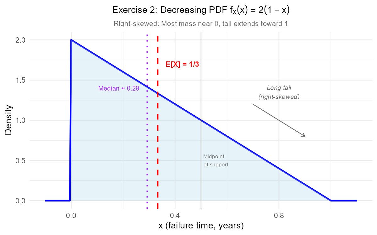
Fig. 6.5 The decreasing PDF \(f_X(x) = 2(1-x)\) is right-skewed with most mass concentrated near 0.

---

Exercise 3: LOTUS with Multiple Functions

An aerospace engineer models aerodynamic drag coefficient \(X\) with PDF:

\[\begin{split}f_X(x) = \begin{cases} \frac{3}{8}x^2, & 0 \leq x \leq 2\\ 0, & \text{elsewhere} \end{cases}\end{split}\]

1. Verify this is a valid PDF.

2. Find \(E[X]\).

3. Find \(E[X^2]\).

4. Find \(E[X^3]\).

5. The power required to overcome drag is proportional to \(X^3\). If \(P = 100X^3\) watts, find \(E[P]\).

6. A naive calculation substitutes \(E[X]\) into the power formula, computing \(g(E[X]) = 100 \cdot (E[X])^3\) instead of \(E[P]\). What value would this give? Which is correct and why do they differ?

Solution

Part (a): Verify PDF validity

Non-negativity: \(\frac{3}{8}x^2 \geq 0\) for all \(x\). ✓

Total area = 1:

\[\int_0^2 \frac{3}{8}x^2 \, dx = \frac{3}{8} \cdot \frac{x^3}{3} \Bigg|_0^2 = \frac{1}{8} \cdot 8 = 1 \text{ ✓}\]

Part (b): E[X]

\[E[X] = \int_0^2 x \cdot \frac{3}{8}x^2 \, dx = \frac{3}{8}\int_0^2 x^3 \, dx = \frac{3}{8} \cdot \frac{x^4}{4} \Bigg|_0^2 = \frac{3}{32} \cdot 16 = \frac{3}{2} = 1.5\]

Part (c): E[X²]

\[E[X^2] = \int_0^2 x^2 \cdot \frac{3}{8}x^2 \, dx = \frac{3}{8}\int_0^2 x^4 \, dx = \frac{3}{8} \cdot \frac{x^5}{5} \Bigg|_0^2 = \frac{3}{40} \cdot 32 = \frac{96}{40} = \frac{12}{5} = 2.4\]

Part (d): E[X³]

\[E[X^3] = \int_0^2 x^3 \cdot \frac{3}{8}x^2 \, dx = \frac{3}{8}\int_0^2 x^5 \, dx = \frac{3}{8} \cdot \frac{x^6}{6} \Bigg|_0^2 = \frac{1}{16} \cdot 64 = 4\]

Part (e): E[P] using LOTUS

Since \(P = 100X^3\):

\[E[P] = E[100X^3] = 100 \cdot E[X^3] = 100 \times 4 = 400 \text{ watts}\]

Part (f): Naive calculation and comparison

The naive calculation substitutes \(E[X]\) directly into the power formula:

\[g(E[X]) = 100 \cdot (E[X])^3 = 100 \cdot (1.5)^3 = 100 \times 3.375 = 337.5 \text{ watts}\]

The correct expected power is 400 watts (from LOTUS).

Why they differ: In general, \(E[g(X)] \neq g(E[X])\) unless \(g\) is a linear function. The power function \(g(x) = 100x^3\) is convex (curves upward for \(x > 0\)), which means \(E[g(X)] > g(E[X])\). Because \(g(x)\) is convex, variability in \(X\) increases the expected value of \(g(X)\).

The naive approach underestimates average power because it ignores variability. Higher-than-average drag coefficients contribute disproportionately to power consumption due to the cubic relationship.

Fig. 6.6 For the convex function \(g(x) = 100x^3\), we have \(E[g(X)] = 400 > g(E[X]) = 337.5\).

---

Exercise 4: Symmetric Distribution and Expected Value

A quality control engineer models measurement error \(X\) (in mm) with PDF:

\[\begin{split}f_X(x) = \begin{cases} \frac{3}{4}(1 - x^2), & -1 \leq x \leq 1\\ 0, & \text{elsewhere} \end{cases}\end{split}\]

1. Verify this is a valid PDF.

2. This PDF is symmetric about \(x = 0\). Use this fact to determine \(E[X]\) without integration.

3. Find \(E[X^2]\).

4. Calculate \(\text{Var}(X)\).

5. Find \(E[X^4]\). (Hint: You’ll need this for problems involving variance of \(X^2\).)

Solution

Part (a): Verify PDF validity

Non-negativity: For \(-1 \leq x \leq 1\), we have \(x^2 \leq 1\), so \(1 - x^2 \geq 0\). Thus \(f_X(x) = \frac{3}{4}(1-x^2) \geq 0\). ✓

Total area = 1:

\[\int_{-1}^{1} \frac{3}{4}(1 - x^2) \, dx = \frac{3}{4}\left[x - \frac{x^3}{3}\right]_{-1}^{1}\]

\[= \frac{3}{4}\left[\left(1 - \frac{1}{3}\right) - \left(-1 + \frac{1}{3}\right)\right] = \frac{3}{4}\left[\frac{2}{3} + \frac{2}{3}\right] = \frac{3}{4} \cdot \frac{4}{3} = 1 \text{ ✓}\]

Part (b): E[X] by symmetry

The PDF \(f_X(x) = \frac{3}{4}(1-x^2)\) is an even function (symmetric about \(x = 0\)):

\[f_X(-x) = \frac{3}{4}(1 - (-x)^2) = \frac{3}{4}(1 - x^2) = f_X(x)\]

When a PDF is symmetric about \(x = c\), the expected value equals \(c\).

Therefore, \(E[X] = 0\).

Part (c): E[X²]

\[E[X^2] = \int_{-1}^{1} x^2 \cdot \frac{3}{4}(1 - x^2) \, dx = \frac{3}{4}\int_{-1}^{1} (x^2 - x^4) \, dx\]

Since \(x^2 - x^4\) is an even function, we can use:

\[= \frac{3}{4} \cdot 2\int_{0}^{1} (x^2 - x^4) \, dx = \frac{3}{2}\left[\frac{x^3}{3} - \frac{x^5}{5}\right]_0^1 = \frac{3}{2}\left(\frac{1}{3} - \frac{1}{5}\right)\]

\[= \frac{3}{2} \cdot \frac{2}{15} = \frac{1}{5} = 0.2\]

Part (d): Var(X)

\[\text{Var}(X) = E[X^2] - (E[X])^2 = \frac{1}{5} - 0^2 = \frac{1}{5} = 0.2\]

\[\sigma_X = \sqrt{0.2} = \frac{1}{\sqrt{5}} \approx 0.447 \text{ mm}\]

Part (e): E[X⁴]

\[E[X^4] = \int_{-1}^{1} x^4 \cdot \frac{3}{4}(1 - x^2) \, dx = \frac{3}{4}\int_{-1}^{1} (x^4 - x^6) \, dx\]

Using symmetry:

\[= \frac{3}{4} \cdot 2\int_{0}^{1} (x^4 - x^6) \, dx = \frac{3}{2}\left[\frac{x^5}{5} - \frac{x^7}{7}\right]_0^1 = \frac{3}{2}\left(\frac{1}{5} - \frac{1}{7}\right)\]

\[= \frac{3}{2} \cdot \frac{2}{35} = \frac{3}{35}\]

Fig. 6.7 The symmetric PDF \(f_X(x) = \frac{3}{4}(1-x^2)\) has \(E[X] = 0\) by symmetry—no integration needed!

---

Exercise 5: Linear Transformations

A chemical engineer measures temperature \(X\) in Celsius with \(E[X] = 25°C\) and \(\sigma_X = 3°C\).

1. Convert to Fahrenheit using \(F = \frac{9}{5}X + 32\). Find \(E[F]\) and \(\sigma_F\).

2. Convert to Kelvin using \(K = X + 273.15\). Find \(E[K]\) and \(\sigma_K\).

3. A control system triggers an alarm when temperature deviates more than 2 standard deviations from the mean. Express this range in all three temperature scales.

4. Why does adding a constant (like 273.15 for Kelvin) not change the standard deviation?

Solution

Part (a): Fahrenheit conversion

Using \(F = \frac{9}{5}X + 32\):

Expected value (linearity):

\[E[F] = E\left[\frac{9}{5}X + 32\right] = \frac{9}{5}E[X] + 32 = \frac{9}{5}(25) + 32 = 45 + 32 = 77°F\]

Standard deviation (variance of linear transformation):

\[\text{Var}(F) = \text{Var}\left(\frac{9}{5}X + 32\right) = \left(\frac{9}{5}\right)^2 \text{Var}(X) = \frac{81}{25} \cdot 9 = \frac{729}{25}\]

\[\sigma_F = \sqrt{\frac{729}{25}} = \frac{27}{5} = 5.4°F\]

Alternatively: \(\sigma_F = \left|\frac{9}{5}\right| \sigma_X = \frac{9}{5} \times 3 = 5.4°F\)

Part (b): Kelvin conversion

Using \(K = X + 273.15\):

Expected value:

\[E[K] = E[X + 273.15] = E[X] + 273.15 = 25 + 273.15 = 298.15 \text{ K}\]

Standard deviation:

\[\text{Var}(K) = \text{Var}(X + 273.15) = 1^2 \cdot \text{Var}(X) = 9\]

\[\sigma_K = 3 \text{ K}\]

The standard deviation is unchanged because adding a constant only shifts the distribution, not its spread.

Part (c): Alarm range (±2σ from mean)

Celsius: \(25 \pm 2(3) = (19, 31)°C\)

Fahrenheit: \(77 \pm 2(5.4) = (66.2, 87.8)°F\)

Kelvin: \(298.15 \pm 2(3) = (292.15, 304.15)\) K

Part (d): Why adding a constant doesn’t change σ

Variance measures spread—how far values deviate from the mean. When we add a constant \(b\) to every value:

• Every observation shifts by the same amount

• The mean also shifts by that same amount

• The deviations from the mean remain unchanged: \((X + b) - (\mu + b) = X - \mu\)

Since variance is based on squared deviations, and those deviations don’t change, variance (and therefore standard deviation) remains the same.

Mathematically: \(\text{Var}(X + b) = E[(X + b - E[X + b])^2] = E[(X - \mu_X)^2] = \text{Var}(X)\)

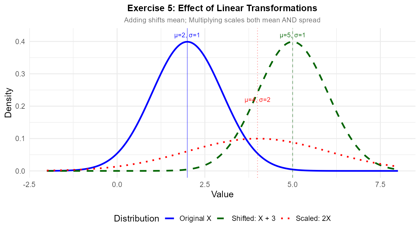
Fig. 6.8 Linear transformations: Adding a constant shifts the mean but preserves spread; multiplying scales both mean and spread.

---

Exercise 6: Sum of Independent Random Variables

A data center has three independent server racks. The power consumption \(X_i\) (in kW) of each rack has \(E[X_i] = 15\) kW and \(\text{Var}(X_i) = 4\) kW².

1. Find the expected total power consumption \(E[X_1 + X_2 + X_3]\).

2. Find \(\text{Var}(X_1 + X_2 + X_3)\) and the standard deviation of total power.

3. The facility has a 50 kW power budget. How many standard deviations above the expected total is this budget?

4. If a fourth identical rack is added, find the new expected total and standard deviation.

5. By what factor does the standard deviation increase when going from 3 to 4 racks? Is this more or less than the factor increase in expected value?

Solution

Part (a): Expected total power

By additivity of expectation:

\[E[X_1 + X_2 + X_3] = E[X_1] + E[X_2] + E[X_3] = 15 + 15 + 15 = 45 \text{ kW}\]

Part (b): Variance and SD of total power

Since the racks are independent, variances add:

\[\text{Var}(X_1 + X_2 + X_3) = \text{Var}(X_1) + \text{Var}(X_2) + \text{Var}(X_3) = 4 + 4 + 4 = 12 \text{ kW}^2\]

\[\sigma_{total} = \sqrt{12} = 2\sqrt{3} \approx 3.46 \text{ kW}\]

Part (c): Budget margin in standard deviations

\[z = \frac{50 - 45}{2\sqrt{3}} = \frac{5}{2\sqrt{3}} = \frac{5\sqrt{3}}{6} \approx 1.44 \text{ standard deviations}\]

The 50 kW budget is about 1.44 standard deviations above the expected consumption.

Part (d): Four racks

Expected total:

\[E[X_1 + X_2 + X_3 + X_4] = 4 \times 15 = 60 \text{ kW}\]

Variance:

\[\text{Var}(X_1 + X_2 + X_3 + X_4) = 4 \times 4 = 16 \text{ kW}^2\]

Standard deviation:

\[\sigma_{\text{total}} = \sqrt{16} = 4 \text{ kW}\]

Part (e): Factor comparison

Standard deviation factor: \(\frac{4}{2\sqrt{3}} = \frac{4}{3.46} \approx 1.155\) (or exactly \(\frac{2}{\sqrt{3}} = \sqrt{\frac{4}{3}}\))

Expected value factor: \(\frac{60}{45} = \frac{4}{3} \approx 1.333\)

The standard deviation increases by a smaller factor than the expected value.

Key insight: For \(n\) independent, identically distributed random variables:

• Expected value of sum = \(n \cdot \mu\) (scales linearly with \(n\))

• Standard deviation of sum = \(\sqrt{n} \cdot \sigma\) (scales with \(\sqrt{n}\))

This “square root law” means that relative variability decreases as we add more independent components—an important principle in risk diversification.

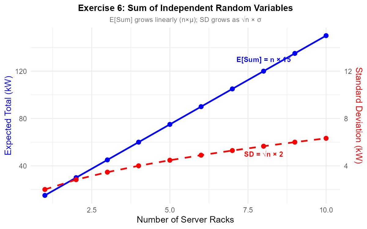
Fig. 6.9 For sums of independent RVs: \(E[\text{Sum}]\) grows linearly with \(n\), while \(\sigma_{\text{Sum}}\) grows as \(\sqrt{n}\).

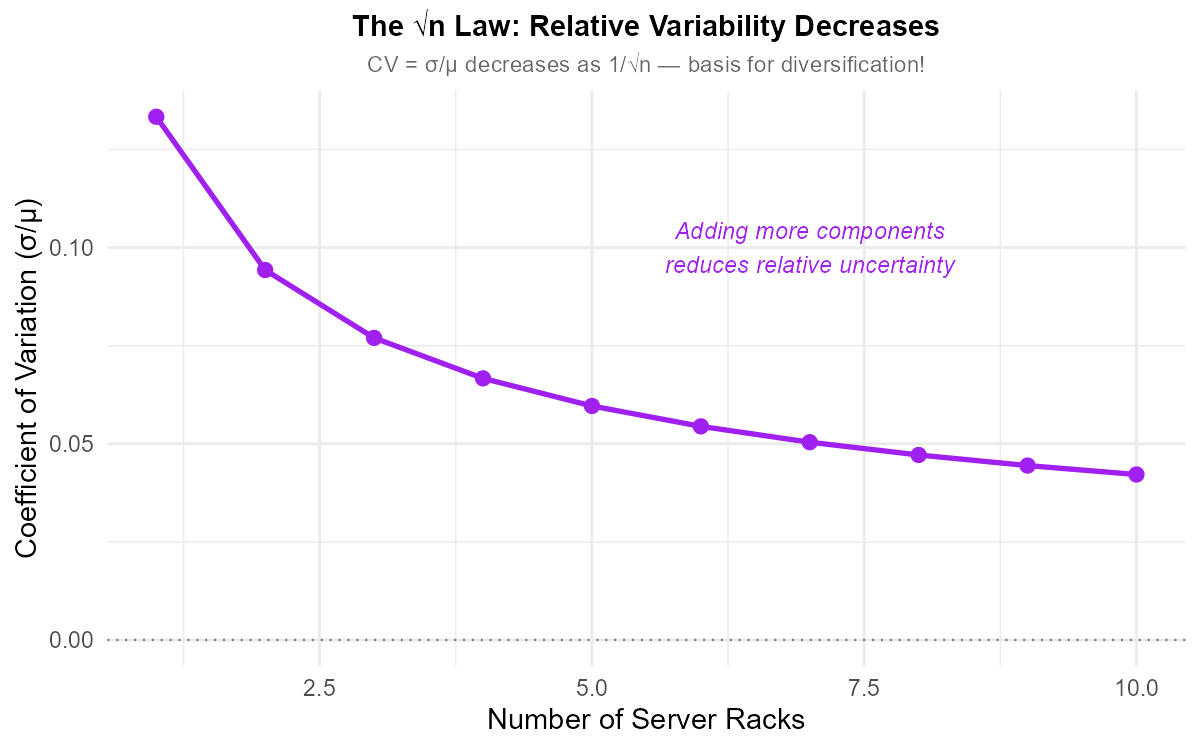
Fig. 6.10 The √n law: Relative variability (CV = σ/μ) decreases as \(1/\sqrt{n}\)—the basis for diversification benefits.

---

Exercise 7: Piecewise PDF with Expected Value

A network engineer models packet sizes \(X\) (in KB) with PDF:

\[\begin{split}f_X(x) = \begin{cases} \frac{x}{4}, & 0 \leq x \leq 2\\ \frac{4-x}{4}, & 2 < x \leq 4\\ 0, & \text{elsewhere} \end{cases}\end{split}\]

1. Verify this is a valid PDF. (Hint: Compute each piece separately.)

2. This is a triangular distribution. Identify its mode (peak).

3. Use symmetry to find \(E[X]\).

4. Find \(E[X^2]\) by computing the integral over both pieces.

5. Calculate \(\text{Var}(X)\).

Solution

Part (a): Verify PDF validity

Non-negativity:

• For \(0 \leq x \leq 2\): \(\frac{x}{4} \geq 0\) ✓

• For \(2 < x \leq 4\): \(4 - x \geq 0\), so \(\frac{4-x}{4} \geq 0\) ✓

Total area = 1:

\[\int_0^2 \frac{x}{4} \, dx + \int_2^4 \frac{4-x}{4} \, dx\]

First integral:

\[\int_0^2 \frac{x}{4} \, dx = \frac{1}{4} \cdot \frac{x^2}{2} \Bigg|_0^2 = \frac{1}{8} \cdot 4 = \frac{1}{2}\]

Second integral:

\[\int_2^4 \frac{4-x}{4} \, dx = \frac{1}{4}\left[4x - \frac{x^2}{2}\right]_2^4 = \frac{1}{4}\left[(16 - 8) - (8 - 2)\right] = \frac{1}{4}(8 - 6) = \frac{1}{2}\]

Total: \(\frac{1}{2} + \frac{1}{2} = 1\) ✓

Part (b): Mode

The mode is where the PDF reaches its maximum. Both pieces meet at \(x = 2\) with \(f_X(2) = \frac{2}{4} = \frac{1}{2}\).

Mode = 2 KB

Part (c): E[X] by symmetry

The triangular PDF is symmetric about \(x = 2\) (the peak).

By symmetry: \(E[X] = 2\) KB

Part (d): E[X²]

\[E[X^2] = \int_0^2 x^2 \cdot \frac{x}{4} \, dx + \int_2^4 x^2 \cdot \frac{4-x}{4} \, dx\]

First integral:

\[\frac{1}{4}\int_0^2 x^3 \, dx = \frac{1}{4} \cdot \frac{x^4}{4} \Bigg|_0^2 = \frac{1}{16} \cdot 16 = 1\]

Second integral:

\[\frac{1}{4}\int_2^4 (4x^2 - x^3) \, dx = \frac{1}{4}\left[\frac{4x^3}{3} - \frac{x^4}{4}\right]_2^4\]

\[= \frac{1}{4}\left[\left(\frac{256}{3} - 64\right) - \left(\frac{32}{3} - 4\right)\right]\]

\[= \frac{1}{4}\left[\frac{256 - 192}{3} - \frac{32 - 12}{3}\right] = \frac{1}{4}\left[\frac{64}{3} - \frac{20}{3}\right] = \frac{1}{4} \cdot \frac{44}{3} = \frac{11}{3}\]

\[E[X^2] = 1 + \frac{11}{3} = \frac{14}{3} \approx 4.67\]

Part (e): Var(X)

\[\text{Var}(X) = E[X^2] - (E[X])^2 = \frac{14}{3} - 4 = \frac{14 - 12}{3} = \frac{2}{3}\]

\[\sigma_X = \sqrt{\frac{2}{3}} = \frac{\sqrt{2}}{\sqrt{3}} = \frac{\sqrt{6}}{3} \approx 0.816 \text{ KB}\]

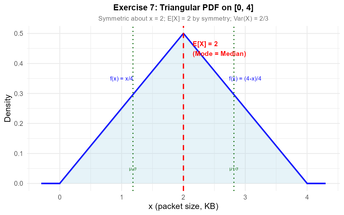
Fig. 6.11 The triangular PDF is symmetric about \(x = 2\), so \(E[X] = 2\) by symmetry.

---

Exercise 8: LOTUS with Non-Polynomial Functions

A materials scientist models crack length \(X\) (in mm) with the uniform PDF:

\[\begin{split}f_X(x) = \begin{cases} 1, & 0 \leq x \leq 1\\ 0, & \text{elsewhere} \end{cases}\end{split}\]

1. Find \(E[X]\) and \(\text{Var}(X)\).

2. Find \(E[\sqrt{X}]\) using LOTUS.

3. Find \(E[e^X]\) using LOTUS.

4. Compare \(E[\sqrt{X}]\) with \(\sqrt{E[X]}\). Which is larger and why?

5. Compare \(E[e^X]\) with \(e^{E[X]}\). Which is larger and why?

Solution

Part (a): E[X] and Var(X)

\[E[X] = \int_0^1 x \cdot 1 \, dx = \frac{x^2}{2} \Bigg|_0^1 = \frac{1}{2}\]

\[E[X^2] = \int_0^1 x^2 \cdot 1 \, dx = \frac{x^3}{3} \Bigg|_0^1 = \frac{1}{3}\]

\[\text{Var}(X) = E[X^2] - (E[X])^2 = \frac{1}{3} - \frac{1}{4} = \frac{1}{12}\]

Part (b): E[√X] using LOTUS

\[E[\sqrt{X}] = \int_0^1 \sqrt{x} \cdot 1 \, dx = \int_0^1 x^{1/2} \, dx = \frac{x^{3/2}}{3/2} \Bigg|_0^1 = \frac{2}{3}\]

Part (c): E[eˣ] using LOTUS

\[E[e^X] = \int_0^1 e^x \cdot 1 \, dx = e^x \Bigg|_0^1 = e - 1 \approx 1.718\]

Part (d): Compare E[√X] with √E[X]

• \(E[\sqrt{X}] = \frac{2}{3} \approx 0.667\)

• \(\sqrt{E[X]} = \sqrt{\frac{1}{2}} = \frac{1}{\sqrt{2}} \approx 0.707\)

\(E[\sqrt{X}] < \sqrt{E[X]}\)

Explanation: The square root function \(g(x) = \sqrt{x}\) is concave (curves downward). For concave functions, we have:

\[E[g(X)] \leq g(E[X])\]

Intuitively: the square root “compresses” larger values more than smaller values, so averaging first (then taking the root) gives a higher result than taking roots first (then averaging).

Part (e): Compare E[eˣ] with e^{E[X]}

• \(E[e^X] = e - 1 \approx 1.718\)

• \(e^{E[X]} = e^{1/2} = \sqrt{e} \approx 1.649\)

\(E[e^X] > e^{E[X]}\)

Explanation: The exponential function \(g(x) = e^x\) is convex (curves upward). For convex functions, we have:

\[E[g(X)] \geq g(E[X])\]

Intuitively: the exponential “amplifies” larger values more than smaller values, so the average of exponentials exceeds the exponential of the average.

Fig. 6.12 Concave function \(g(x) = \sqrt{x}\): \(E[g(X)] \leq g(E[X])\).

Fig. 6.13 Convex function \(g(x) = e^x\): \(E[g(X)] \geq g(E[X])\).

---

Exercise 9: Variance of a Transformed Variable

A computer scientist models algorithm runtime \(X\) (in seconds) with PDF:

\[\begin{split}f_X(x) = \begin{cases} 2x, & 0 \leq x \leq 1\\ 0, & \text{elsewhere} \end{cases}\end{split}\]

1. Find \(E[X]\), \(E[X^2]\), and \(\text{Var}(X)\).

2. The cost function is \(C = 5X + 10\) dollars. Find \(E[C]\) and \(\text{Var}(C)\).

3. A quadratic cost model uses \(Q = 3X^2\). Find \(E[Q]\).

4. For the quadratic cost \(Q = 3X^2\), find \(\text{Var}(Q)\). (Hint: You need \(E[X^4]\).)

Solution

Part (a): Basic moments

\[E[X] = \int_0^1 x \cdot 2x \, dx = 2\int_0^1 x^2 \, dx = 2 \cdot \frac{1}{3} = \frac{2}{3}\]

\[E[X^2] = \int_0^1 x^2 \cdot 2x \, dx = 2\int_0^1 x^3 \, dx = 2 \cdot \frac{1}{4} = \frac{1}{2}\]

\[\text{Var}(X) = E[X^2] - (E[X])^2 = \frac{1}{2} - \frac{4}{9} = \frac{9 - 8}{18} = \frac{1}{18}\]

Part (b): Linear cost C = 5X + 10

Using linearity of expectation:

\[E[C] = E[5X + 10] = 5E[X] + 10 = 5 \cdot \frac{2}{3} + 10 = \frac{10}{3} + 10 = \frac{40}{3} \approx \$13.33\]

Using variance of linear transformation:

\[\text{Var}(C) = \text{Var}(5X + 10) = 5^2 \cdot \text{Var}(X) = 25 \cdot \frac{1}{18} = \frac{25}{18} \approx 1.39\]

\[\sigma_C = \sqrt{\frac{25}{18}} = \frac{5}{3\sqrt{2}} \approx \$1.18\]

Part (c): Quadratic cost Q = 3X²

Note: \(Q\) is defined as a cost in dollars, where the coefficient 3 carries units of dollars/second² to ensure dimensional consistency.

Using LOTUS:

\[E[Q] = E[3X^2] = 3 \cdot E[X^2] = 3 \cdot \frac{1}{2} = \frac{3}{2} = \$1.50\]

Part (d): Var(Q) for Q = 3X²

We need \(E[Q^2] = E[9X^4] = 9E[X^4]\).

First, find \(E[X^4]\):

\[E[X^4] = \int_0^1 x^4 \cdot 2x \, dx = 2\int_0^1 x^5 \, dx = 2 \cdot \frac{1}{6} = \frac{1}{3}\]

Now:

\[E[Q^2] = 9 \cdot E[X^4] = 9 \cdot \frac{1}{3} = 3\]

\[\text{Var}(Q) = E[Q^2] - (E[Q])^2 = 3 - \left(\frac{3}{2}\right)^2 = 3 - \frac{9}{4} = \frac{3}{4}\]

\[\sigma_Q = \sqrt{\frac{3}{4}} = \frac{\sqrt{3}}{2} \approx \$0.87\]

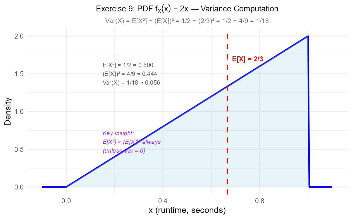
Fig. 6.14 The variance shortcut: \(\text{Var}(X) = E[X^2] - (E[X])^2\). Note that \(E[X^2] > (E[X])^2\) always (unless Var = 0).

---

6.2.9. Additional Practice Problems

True/False Questions (1 point each)

1. For a continuous random variable, \(E[X^2] = (E[X])^2\).

   Ⓣ or Ⓕ

2. If \(X\) has PDF symmetric about \(x = 5\), then \(E[X] = 5\).

   Ⓣ or Ⓕ

3. For any random variable \(X\) and constant \(c\), \(\text{Var}(X + c) = \text{Var}(X)\).

   Ⓣ or Ⓕ

4. If \(X\) and \(Y\) are independent, then \(\text{Var}(X + Y) = \text{Var}(X) + \text{Var}(Y)\).

   Ⓣ or Ⓕ

5. \(E[3X + 2] = 3E[X] + 2\) is an example of the linearity of expectation.

   Ⓣ or Ⓕ

6. For any function \(g(x)\), \(E[g(X)] = g(E[X])\).

   Ⓣ or Ⓕ

7. Variance can never be negative.

   Ⓣ or Ⓕ

8. If \(\text{Var}(X) = 9\), then \(\text{Var}(2X) = 18\).

   Ⓣ or Ⓕ

Multiple Choice Questions (2 points each)

9. For \(f_X(x) = 2x\) on \([0, 1]\), what is \(E[X]\)?

   Ⓐ 1/3

   Ⓑ 1/2

   Ⓒ 2/3

   Ⓓ 3/4

10. If \(E[X] = 4\) and \(E[X^2] = 20\), what is \(\text{Var}(X)\)?

    Ⓐ 4

    Ⓑ 16

    Ⓒ 20

    Ⓓ 36

11. If \(\text{Var}(X) = 5\), what is \(\text{Var}(3X - 7)\)?

    Ⓐ 5

    Ⓑ 8

    Ⓒ 15

    Ⓓ 45

12. If \(X\) and \(Y\) are independent with \(\text{Var}(X) = 3\) and \(\text{Var}(Y) = 5\), what is \(\text{Var}(X + Y)\)?

    Ⓐ 2

    Ⓑ 8

    Ⓒ 15

    Ⓓ 64

13. For \(f_X(x) = 3x^2\) on \([0, 1]\), what is \(E[X^2]\)?

    Ⓐ 1/2

    Ⓑ 3/5

    Ⓒ 3/4

    Ⓓ 4/5

14. Which property allows us to compute \(E[X^2]\) directly from \(f_X(x)\) without finding the PDF of \(X^2\)?

    Ⓐ Linearity of expectation

    Ⓑ Additivity of variance

    Ⓒ Law of the Unconscious Statistician (LOTUS)

    Ⓓ Variance shortcut formula

Answers to Practice Problems

True/False Answers:

1. False — In general, \(E[X^2] \geq (E[X])^2\). Equality holds only when \(\text{Var}(X) = 0\) (i.e., \(X\) is a constant).

2. True — Symmetry about \(x = c\) implies \(E[X] = c\) (the balance point).

3. True — Adding a constant shifts all values but doesn’t change the spread. \(\text{Var}(X + c) = \text{Var}(X)\).

4. True — For independent random variables, variances add: \(\text{Var}(X + Y) = \text{Var}(X) + \text{Var}(Y)\).

5. True — This is exactly the linearity property: \(E[aX + b] = aE[X] + b\).

6. False — In general, \(E[g(X)] \neq g(E[X])\) unless \(g\) is linear. This is why LOTUS is needed.

7. True — Variance is \(E[(X - \mu)^2]\), an expected value of squared terms, which cannot be negative.

8. False — \(\text{Var}(2X) = 2^2 \cdot \text{Var}(X) = 4 \times 9 = 36\), not 18.

Multiple Choice Answers:

9. Ⓒ — \(E[X] = \int_0^1 x \cdot 2x \, dx = 2 \cdot \frac{1}{3} = \frac{2}{3}\).

10. Ⓐ — \(\text{Var}(X) = E[X^2] - (E[X])^2 = 20 - 16 = 4\).

11. Ⓓ — \(\text{Var}(3X - 7) = 3^2 \cdot \text{Var}(X) = 9 \times 5 = 45\).

12. Ⓑ — For independent RVs: \(\text{Var}(X + Y) = \text{Var}(X) + \text{Var}(Y) = 3 + 5 = 8\).

13. Ⓑ — \(E[X^2] = \int_0^1 x^2 \cdot 3x^2 \, dx = 3 \cdot \frac{1}{5} = \frac{3}{5}\).

14. Ⓒ — LOTUS (Law of the Unconscious Statistician) allows \(E[g(X)] = \int g(x) f_X(x) \, dx\) directly.