Slides 📊

Download Chapter 12 slides (PPTX)

12.2. Different Sources of Variability in ANOVA

In our previous exploration using side-by-side boxplots, we learned that comparing means in isolation was not sufficient—we had to consider how much variability existed within each group in comparison with the spread of the group means. In this lesson, we formalize this idea mathematically.

Road Map 🧭

• Identify the three sources of variability in ANOVA. Quantify the variability from each source using formal notation.

• Recognize the roles of sum of squares, degrees of freedom and mean of squares in constructing a sample variance.

• Learn the special relationship between the three sums of squares and their degrees of freedom.

• Organize the components into an ANOVA table.

12.2.1. The One-Way ANOVA Model

What is a Statistical Model?

As we progress to statistical inference methods of higher complexity, it becomes essential to define a corresponding statistical model to concisely express the core ideas. A statistical model provides a structural decomposition of the data that must hold under the assumptions of the analysis method.

The One-Way ANOVA Model

One-way ANOVA assumes that an observation \(X_{ij}\) takes the following form:

\[X_{ij} = \mu_i + \varepsilon_{ij}.\]

Anove, \(\mu_{i}\) is the unknown true mean of Group \(i\), and \(\varepsilon_{ij}\) is the random error that captures everything not explained by the group mean.

According to the ANOVA assumptions, the random errors are mutually independent and have an equal variance of \(\sigma^2\). Since we have extracted the group means out of the random term, \(\varepsilon_{ij}\) would also have an expected value of zero.

In the ideal case where all populations are normally distributed, therefore, we can write:

\[\varepsilon_{ij} \sim_{iid} N(0, \sigma^2)\]

Why Is the Model Helpful?

The ANOVA model allows us to view each data point as the outcome of two components, each contributing distinctly. If all population means are truly equal, the only source of randomness among observations would be the \(\varepsilon_{ij}\) terms, whose variance is \(\sigma^2\). If the observed variance in the data is significantly larger than \(\sigma^2\), therefore, we must consider the possibility that differences in group means also contribute.

To formalize this, we first construct the three key measures of variation in ANOVA: variation between groups, variation within groups, and the total variation.

12.2.2. Three Types of Variability

As with any sample variance we have seen before, the three measures of variation will take the following common form:

\[S^2 = \frac{\text{Sum of Squares}}{\text{df}},\]

where the degrees of freedom are chosen to make each statistic an unbiased estimator of its target. The degrees of freedom will show the pattern we have previously seen—it is equal to the difference between the number of data points and the number of estimated means used for construction of the statistic.

Since each sample variance of this form is an “average” of squares, we also call them a mean of squares (MS).

1. SSA and MSA: Between-Group Variation

We first consider the sum of sqaures for between-group variation, or SSA.

\[\text{SSA} = \sum_{i=1}^k n_i (\bar{X}_{i \cdot} - \bar{X}_{\cdot \cdot})^2\]

Note that SSA is the sum of squared deviations of group means from the overall mean, each weighted proportionally to the group size. The degrees of freedom appropriate for SSA is \(df_A = k-1\) since there are \(k\) group means deviating from a single overall mean.

It follows that the mean of squares for the variation between groups is:

\[\text{MSA} = \frac{\text{SSA}}{df_A} = \frac{\sum_{i=1}^k n_i (\bar{X}_{i \cdot} - \bar{X}_{\cdot \cdot})^2}{k-1}.\]

MSA has a special property:

• If \(H_0\) is true and the equal variance assumption holds, then the MSA is an unbiased estimator of \(\sigma^2\).

• However, if \(H_0\) is false, then the MSA estimates \(\sigma^2\) plus additional variation due to differences in population means.

Therefore, an MSA significantly larger than an estimate of \(\sigma^2\) indicates the existence of additional variance due to distinct group means, whereas an MSA comparable to an estimated \(\sigma^2\) indicates an absence of strong evidence against the null hypothesis.

Why Do We call It SS”A”?

The name SSA stands for “Sum of Squares for Factor A”. It originates from the multi-way ANOVA context involving multiple factors (Factor A, Factor B, etc.). By convention, the sum of squares for the “first” factor is labeled SSA, even when there is only one factor in the anlaysis.

Example 💡: Coffeehouse SSA & MSA ☕️

In the coffeehouse example, SSA and MSA measure how much the store-wise average ages vary from the overall mean. If all the coffeehouses attract similar demographics, SSA and MSA should be small. If they attract different age groups, they should be large.

2. SSE and MSE: Within-Group Variation

The sum of squares of errors, or SSE, is an unscaled measure of how observations within each group deviate from their respective group means due to the random error, \(\varepsilon_{ij}\).

\[\text{SSE} = \sum_{i=1}^k \sum_{j=1}^{n_i} (X_{ij} - \bar{X}_{i \cdot})^2 = \sum_{i=1}^k (n_i - 1) S^2_{i\cdot}\]

Confirm the second equality by replacing \(S^2_{i\cdot}\) with its explicit formula. The SSE consists of the squared distances of \(n\) observations from one of \(k\) group means, giving us the degrees of freedom \(df_E=n-k\).

Bringing SSE to the correct scale with the degrees of freedom, we obtain:

\[\text{MSE} = \frac{\text{SSE}}{df_E} = \frac{\sum_{i=1}^k \sum_{j=1}^{n_i} (X_{ij} - \bar{X}_{i \cdot})^2}{n-k}.\]

MSE is an unbiased estimator of the variance within populations, \(\sigma^2\), regardless of whether \(H_0\) is true. As a result, we always estimate the within-population variance with \(S^2 = MSE\). The estimator for population-wise standard deviation is \(S= \sqrt{MSE}\).

Connecting ANOVA and Indepdent Two-Sample Analysis

MSE is a multi-way extension of the pooled variance estimator for independent two-sample analysis. Confirm this by plugging in \(k=2\) to recover \(S^2_p\).

Example 💡: Coffeehouse SSE & MSE ☕️

In the coffeehouse example, the SSE and MSE measure how much individual customer ages vary within each coffeehouse. They represent the natural variation in customer ages that exists regardless of any systematic differences between coffeehouses.

3. Total Sum of Squares (SST)

Finally, we also define a measure for the overall variability in the data.

\[\text{SST} = \sum_{i=1}^k \sum_{j=1}^{n_i} (X_{ij} - \bar{X}_{\cdot \cdot})^2\]

Note that this would be the numerator for the sample variance if the entire dataset was treated as a single sample. The distances of \(n\) total observations are measured against one overall mean estimator, giving us the degrees of freedom \(df_T = n - 1\).

We do not define a mean of sqaures for the total variation, as it does not hold significance in the ANOVA framework.

Example 💡: Coffeehouse SST ☕️

In the coffeehouse example, SST measures the degree of variation of all customer ages around the single overall sample mean.

12.2.3. The Fundamental ANOVA Identity

The remarkable mathematical result that makes ANOVA possible is that the sums of squares are related by:

\[\text{SST} = \text{SSA} + \text{SSE}\]

Moreover, the degrees of freedom decompose in the same way:

\[(n - 1) = (k - 1) + (n - k)\]

Why This Decomposition Works

We use the trick of adding and subtracting the same terms inside each pair of parentheses in SST:

\[\begin{split}\text{SST} &= \sum_{i=1}^k \sum_{j=1}^{n_i} (X_{ij} - \bar{X}_{\cdot \cdot})^2 \\ &= \sum_{i=1}^k \sum_{j=1}^{n_i} [(X_{ij} - \bar{X}_{i \cdot}) + (\bar{X}_{i \cdot} - \bar{X}_{\cdot \cdot})]^2\\ &= \sum_{i=1}^k \sum_{j=1}^{n_i} [(X_{ij} - \bar{X}_{i \cdot})^2 + (\bar{X}_{i \cdot} - \bar{X}_{\cdot \cdot})^2 + 2(X_{ij} - \bar{X}_{i \cdot})(\bar{X}_{i \cdot} - \bar{X}_{\cdot \cdot})] \\ &= SSE + SSA + \sum_{i=1}^k \sum_{j=1}^{n_i}2(X_{ij} - \bar{X}_{i \cdot})(\bar{X}_{i \cdot} - \bar{X}_{\cdot \cdot})\end{split}\]

The cross-product term can be shown to equal zero by taking the following steps:

• Since \(2(\bar{X}_{i \cdot} - \bar{X}_{\cdot \cdot})\) does not depend on \(j\), we can factor it out of the inner sum.

• The inner sum is then

  \[\sum_{j=1}^{n_i} (X_{ij} - \bar{X}_{i \cdot}) = \sum_{j=1}^{n_i}X_{ij} - n_{i}\cdot\frac{\sum_{j=1}^{n_i}X_{ij}}{n_i} = 0.\]

12.2.4. The ANOVA Table

The components of ANOVA are often organized into a table, with rows representing the three difference sources of variability, and the columns representing various characteristics of each source.

Source	df	SS	MS	F	\(p\)-value
Factor A	\(k-1\)	\(\sum_{i=1}^k n_i(\bar{x}_{i \cdot} - \bar{x}_{\cdot \cdot})^2\)	\(\frac{\text{SSA}}{k-1}\)	?	?
Error	\(n-k\)	\(\sum_{i=1}^k \sum_{j=1}^{n_i}(x_{ij} - \bar{x}_{i \cdot})^2\)	\(\frac{\text{SSE}}{n-k}\)
Total	\(n-1\)	\(\sum_{i=1}^k \sum_{j=1}^{n_i}(x_{ij} - \bar{x}_{\cdot \cdot})^2\)

The total row is often omitted for conciseness as their entries can be computed by adding up the other dfs and the sums of squares. The entries corresponding to \(F\) and \(p\)-value will be discussed in the upcoming lesson.

Example 💡: Coffeehouse ANOVA Table ☕️

Using the data summary and the partial ANOVA table of the coffeehouse example,

• Fill in the blank entries of the ANOVA table.

• Provide an estimate of the population standard deviation, \(\sigma\).

📊 Download the coffeehouse dataset (CSV)

Data Summary

Table 12.2 Sample Statistics

Sample (Levels of Factor Variable)	Sample Size	Mean	Variance
Population 1	\(n_1 = 39\)	\(\bar{x}_{1.} = 39.13\)	\(s_1^2 = 62.43\)
Population 2	\(n_2 = 38\)	\(\bar{x}_{2.} = 46.66\)	\(s_2^2 = 168.34\)
Population 3	\(n_3 = 42\)	\(\bar{x}_{3.} = 40.50\)	\(s_3^2 = 119.62\)
Population 4	\(n_4 = 38\)	\(\bar{x}_{4.} = 26.42\)	\(s_4^2 = 48.90\)
Population 5	\(n_5 = 43\)	\(\bar{x}_{5.} = 34.07\)	\(s_5^2 = 98.50\)
Combined	\(n = 200\)	\(\bar{x}_{..} = 37.35\)	\(s^2 = 142.14\)

Partially Complete ANOVA Table

Source	df	SS	MS
Factor A	(1)	(4)	(6)
Error	(2)	(5)	99.8
Total	(3)	28285

Let us begin with the degrees of freedom since they can be obtained directly from the data summary. We have \(n=200\) and \(k=5\). Therefore,

• (1) \(df_A = k - 1 = 4\)

• (2) \(df_E = n - k = 200 - 5 = 195\)

• (3) \(df_T = n - 1 = 199\)

We can use \(df_T = df_A + df_E\) as a second check.

(5) \(MSE = 99.8 = \frac{SSE}{195}\), so

\[SSE = 99.8 \times 195 = 19461\]

(4) Then, using the fact that SSA and SSE add up to SST,

\[SSA = SST - SSE = 28285 - 19461 = 8834\]

(6) Finally,

\[MSA = \frac{SSA}{df_A} = \frac{8824}{4} = 2208.4\]

The MSE as a random variable is an unbiased estimator of \(\sigma^2\). We can use the square root of its observed value as an estimate for \(\sigma\).

\[\hat{\sigma} = \sqrt{MSE} = \sqrt{99.8} = 9.99\]

12.2.5. Bringing It All Together

Key Takeaways 📝

1. The ANOVA model decomposes each observation into a group effect plus random error: \(X_{ij} = \mu_i + \varepsilon_{ij}\).

2. Total Sum of Squares (SST) satisfies \(SST = SSA + SSE\). Their degrees of freedom have a similar association: \(df_T = df_A + df_E\).

3. Since \(E(MSE) = \sigma^2\) always holds, we use the MSE as the estimator of the common variance \(\sigma^2\), and also denote its observed value as \(s^2\).

4. MSA is an unbiased astimator of \(\sigma^2\) only when \(H_0\) is true —its true target is greater than \(\sigma^2\) when \(H_0\) is false. Therefore, comparing MSA against MSE gives us a measure of data evidence against the null hypothesis.

12.2.6. Exercises

Exercise 1: Computing the Overall Mean

A quality engineer compares the tensile strength (in MPa) of welds produced by four different welding techniques. Summary statistics are:

Technique	Sample Size	Mean Strength
MIG (Group 1)	12	485.2
TIG (Group 2)	15	492.8
Stick (Group 3)	10	478.5
Flux-cored (Group 4)	13	488.1

1. Calculate the total sample size \(n\).

2. Calculate the overall (grand) mean \(\bar{x}_{..}\) using the weighted average formula.

3. Verify that the grand mean is NOT simply the average of the four group means. Why does this matter?

Solution

Part (a): Total sample size

\[n = n_1 + n_2 + n_3 + n_4 = 12 + 15 + 10 + 13 = 50\]

Part (b): Overall mean

The grand mean is a weighted average of group means:

\[\bar{x}_{..} = \frac{\sum_{i=1}^{k} n_i \bar{x}_{i.}}{n} = \frac{12(485.2) + 15(492.8) + 10(478.5) + 13(488.1)}{50}\]

\[= \frac{5822.4 + 7392 + 4785 + 6345.3}{50} = \frac{24344.7}{50} = 486.89 \text{ MPa}\]

Part (c): Comparison with simple average

Simple average of group means:

\[\frac{485.2 + 492.8 + 478.5 + 488.1}{4} = \frac{1944.6}{4} = 486.15 \text{ MPa}\]

The weighted mean (486.89) differs from the simple average (486.15) because groups have unequal sample sizes. Groups with larger n contribute more to the overall mean. This matters because:

• TIG (n=15, highest mean) pulls the weighted average up

• Stick (n=10, lowest mean) has less influence

• Using the wrong formula would lead to incorrect SSA calculations

R verification:

n <- c(12, 15, 10, 13)
xbar <- c(485.2, 492.8, 478.5, 488.1)

n_total <- sum(n)  # 50
grand_mean <- sum(n * xbar) / n_total  # 486.894
simple_avg <- mean(xbar)  # 486.15

---

Exercise 2: Computing SSA (Between-Group Variation)

Using the welding data from Exercise 1 (with \(\bar{x}_{..} = 486.89\) MPa):

1. Write out the formula for SSA and explain what each component represents.

2. Calculate SSA step by step.

3. Calculate the degrees of freedom for SSA (\(df_A\)).

4. Calculate MSA.

5. Interpret what a large MSA would indicate about the welding techniques.

Solution

Part (a): SSA formula

\[\text{SSA} = \sum_{i=1}^{k} n_i (\bar{x}_{i.} - \bar{x}_{..})^2\]

Components:

• \(n_i\) = sample size for group i (weights each group’s contribution)

• \(\bar{x}_{i.}\) = sample mean for group i

• \(\bar{x}_{..}\) = overall grand mean

• \((\bar{x}_{i.} - \bar{x}_{..})^2\) = squared deviation of group mean from grand mean

SSA measures how much the group means vary around the overall mean.

Part (b): SSA calculation

First, compute each group’s contribution:

Group	\(n_i\)	\(\bar{x}_{i.}\)	\(\bar{x}_{i.} - \bar{x}_{..}\)	\(n_i(\bar{x}_{i.} - \bar{x}_{..})^2\)
MIG	12	485.2	-1.69	34.29
TIG	15	492.8	5.91	523.87
Stick	10	478.5	-8.39	703.92
Flux-cored	13	488.1	1.21	19.04

\[\text{SSA} = 34.29 + 523.87 + 703.92 + 19.04 = 1281.12\]

Part (c): Degrees of freedom

\[df_A = k - 1 = 4 - 1 = 3\]

Part (d): MSA calculation

\[\text{MSA} = \frac{\text{SSA}}{df_A} = \frac{1281.12}{3} = 427.04\]

Part (e): Interpretation

A large MSA indicates that the group means are spread widely around the grand mean—suggesting that the welding techniques produce systematically different tensile strengths. If MSA is significantly larger than MSE (the within-group variability), this provides evidence that at least one technique differs from the others.

R verification:

n <- c(12, 15, 10, 13)
xbar <- c(485.2, 492.8, 478.5, 488.1)
grand_mean <- sum(n * xbar) / sum(n)  # 486.894

SSA <- sum(n * (xbar - grand_mean)^2)  # 1281.12
df_A <- length(n) - 1  # 3
MSA <- SSA / df_A  # 427.04

---

Exercise 3: Computing SSE (Within-Group Variation)

Continuing with the welding data, the sample standard deviations for each technique are:

Technique	\(n_i\)	\(\bar{x}_{i.}\)	\(s_i\)
MIG	12	485.2	8.5
TIG	15	492.8	7.2
Stick	10	478.5	9.8
Flux-cored	13	488.1	8.1

1. Write the formula for SSE and explain its relationship to the individual group variances.

2. Calculate SSE using the shortcut formula \(\text{SSE} = \sum_{i=1}^{k}(n_i - 1)s_i^2\).

3. Calculate \(df_E\) and MSE.

4. Provide an estimate of the common population standard deviation \(\sigma\).

5. Check the equal variance assumption using the rule of thumb.

Solution

Part (a): SSE formula

\[\text{SSE} = \sum_{i=1}^{k} \sum_{j=1}^{n_i} (x_{ij} - \bar{x}_{i.})^2 = \sum_{i=1}^{k}(n_i - 1)s_i^2\]

The shortcut works because \(s_i^2 = \frac{\sum_{j=1}^{n_i}(x_{ij} - \bar{x}_{i.})^2}{n_i - 1}\), so multiplying by \((n_i - 1)\) recovers the sum of squares for each group.

SSE measures the total variability within all groups—variation that cannot be explained by group membership.

Part (b): SSE calculation

Group	\(n_i - 1\)	\(s_i^2\)	\((n_i - 1)s_i^2\)
MIG	11	72.25	794.75
TIG	14	51.84	725.76
Stick	9	96.04	864.36
Flux-cored	12	65.61	787.32

\[\text{SSE} = 794.75 + 725.76 + 864.36 + 787.32 = 3172.19\]

Part (c): df_E and MSE

\[df_E = n - k = 50 - 4 = 46\]

\[\text{MSE} = \frac{\text{SSE}}{df_E} = \frac{3172.19}{46} = 68.96\]

Part (d): Estimate of σ

\[\hat{\sigma} = \sqrt{\text{MSE}} = \sqrt{68.96} = 8.30 \text{ MPa}\]

This is our best estimate of the common within-group standard deviation.

Part (e): Equal variance check

\[\frac{\max(s_i)}{\min(s_i)} = \frac{9.8}{7.2} = 1.36\]

Since 1.36 ≤ 2, the equal variance assumption is satisfied ✓

R verification:

n <- c(12, 15, 10, 13)
s <- c(8.5, 7.2, 9.8, 8.1)

SSE <- sum((n - 1) * s^2)  # 3172.19
df_E <- sum(n) - length(n)  # 46
MSE <- SSE / df_E  # 68.96
sigma_hat <- sqrt(MSE)  # 8.30

max(s) / min(s)  # 1.36 - passes rule of thumb

---

Exercise 4: The Fundamental ANOVA Identity

The fundamental ANOVA identity states: \(\text{SST} = \text{SSA} + \text{SSE}\).

1. Using SSA = 1281.12 and SSE = 3172.19 from the previous exercises, calculate SST.

2. Verify the degrees of freedom relationship: \(df_T = df_A + df_E\).

3. If you were given SST = 5000 and SSA = 1500, what would SSE be?

4. Explain why MST (if we computed it) would NOT equal MSA + MSE, even though SST = SSA + SSE.

Solution

Part (a): Calculate SST

\[\text{SST} = \text{SSA} + \text{SSE} = 1281.12 + 3172.19 = 4453.31\]

Part (b): Verify df relationship

• \(df_A = k - 1 = 3\)

• \(df_E = n - k = 46\)

• \(df_T = n - 1 = 49\)

Check: \(df_A + df_E = 3 + 46 = 49 = df_T\) ✓

Part (c): Finding SSE from SST and SSA

\[\text{SSE} = \text{SST} - \text{SSA} = 5000 - 1500 = 3500\]

Part (d): Why MS doesn’t add

Mean squares are sums of squares divided by their respective degrees of freedom:

• \(\text{MSA} = \frac{\text{SSA}}{df_A}\)

• \(\text{MSE} = \frac{\text{SSE}}{df_E}\)

• \(\text{MST} = \frac{\text{SST}}{df_T}\) (if computed)

Even though SST = SSA + SSE, dividing by different denominators breaks the additive relationship:

\[\text{MST} = \frac{\text{SST}}{df_T} = \frac{\text{SSA} + \text{SSE}}{df_A + df_E} \neq \frac{\text{SSA}}{df_A} + \frac{\text{SSE}}{df_E}\]

This is analogous to why \(\frac{a+b}{c+d} \neq \frac{a}{c} + \frac{b}{d}\) in general.

---

Exercise 5: Completing a Partial ANOVA Table

An aerospace engineer tests the fatigue life (in thousands of cycles) of turbine blades made from three different alloys. The partial ANOVA table is:

Source	df	SS	MS
Alloy	(a)	(d)	845.6
Error	(b)	2536.8	(e)
Total	(c)	4228.0

The study used 12 blades from each of the 3 alloys.

Complete all missing entries (a) through (e).

Solution

Given information:

• k = 3 alloys

• n_i = 12 for each alloy → n = 36 total

• MSA = 845.6

• SSE = 2536.8

• SST = 4228.0

Step 1: Degrees of freedom

(a) \(df_A = k - 1 = 3 - 1 = 2\)

(b) \(df_E = n - k = 36 - 3 = 33\)

(c) \(df_T = n - 1 = 35\)

Verification: \(2 + 33 = 35\) ✓

Step 2: Calculate SSA

From \(\text{MSA} = \frac{\text{SSA}}{df_A}\):

(d) \(\text{SSA} = \text{MSA} \times df_A = 845.6 \times 2 = 1691.2\)

Verification: SSA + SSE = 1691.2 + 2536.8 = 4228.0 = SST ✓

Step 3: Calculate MSE

(e) \(\text{MSE} = \frac{\text{SSE}}{df_E} = \frac{2536.8}{33} = 76.87\)

Complete ANOVA Table:

Source	df	SS	MS
Alloy	2	1691.2	845.6
Error	33	2536.8	76.87
Total	35	4228.0

R verification:

k <- 3
n <- 36
MSA <- 845.6
SSE <- 2536.8
SST <- 4228.0

df_A <- k - 1  # 2
df_E <- n - k  # 33
df_T <- n - 1  # 35

SSA <- MSA * df_A  # 1691.2
MSE <- SSE / df_E  # 76.87

# Verification
SSA + SSE  # Should equal SST = 4228

---

Exercise 6: MSE as the Pooled Variance Estimator

This exercise connects ANOVA to the pooled variance from Chapter 11.

1. Write the formula for the pooled variance estimator \(s_p^2\) from two-sample inference (Chapter 11).

2. Write the formula for MSE in ANOVA.

3. Show that when k = 2, MSE reduces to \(s_p^2\).

4. Why is this connection important?

Solution

Part (a): Pooled variance from Chapter 11

For two independent samples:

\[s_p^2 = \frac{(n_A - 1)s_A^2 + (n_B - 1)s_B^2}{n_A + n_B - 2}\]

Part (b): MSE formula

\[\text{MSE} = \frac{\text{SSE}}{n - k} = \frac{\sum_{i=1}^{k}(n_i - 1)s_i^2}{n - k}\]

Part (c): Showing MSE = s_p² when k = 2

When k = 2, let the groups be A and B:

\[\text{MSE} = \frac{(n_A - 1)s_A^2 + (n_B - 1)s_B^2}{(n_A + n_B) - 2} = \frac{(n_A - 1)s_A^2 + (n_B - 1)s_B^2}{n_A + n_B - 2}\]

This is exactly the formula for \(s_p^2\)!

Part (d): Why this matters

This connection shows that:

1. ANOVA generalizes two-sample methods: MSE extends the pooled variance concept to k ≥ 2 groups

2. Consistent variance estimation: Whether using two-sample t-tests or ANOVA, we use the same approach—pooling information from all groups to estimate the common variance

3. Unified framework: ANOVA with k = 2 is mathematically equivalent to the pooled two-sample t-test (as we’ll see in Section 12.3)

4. Equal variance assumption: Both methods assume equal population variances; MSE is only an unbiased estimator of σ² when this assumption holds

---

Exercise 7: Interpreting Sums of Squares

A computer scientist compares the runtime (in seconds) of sorting algorithms on datasets of similar size. After collecting data:

• SSA = 2450 (between-algorithm variability)

• SSE = 1890 (within-algorithm variability)

• k = 5 algorithms

• n = 60 total test runs

1. What proportion of the total variability is explained by differences between algorithms?

2. What proportion is due to random variation within algorithms?

3. Based on these proportions alone (without a formal test), do you expect differences between algorithms to be statistically significant? Explain.

4. Calculate MSA and MSE. What does the ratio MSA/MSE suggest?

Solution

Part (a): Proportion explained by algorithms

First, calculate SST:

\[\text{SST} = \text{SSA} + \text{SSE} = 2450 + 1890 = 4340\]

Proportion explained by between-group differences:

\[\frac{\text{SSA}}{\text{SST}} = \frac{2450}{4340} = 0.565 = 56.5\%\]

Part (b): Proportion due to within-group variation

\[\frac{\text{SSE}}{\text{SST}} = \frac{1890}{4340} = 0.435 = 43.5\%\]

(Or simply: 100% - 56.5% = 43.5%)

Part (c): Prediction about significance

With 56.5% of variation attributable to algorithm differences, there’s a good chance the F-test will be significant. The between-group variability is larger than the within-group variability, which is the pattern we’d expect when group means truly differ.

However, we need the formal F-test to account for degrees of freedom and determine if this proportion is large enough to be statistically significant at a given α level.

Part (d): MSA/MSE ratio

\[df_A = k - 1 = 4, \quad df_E = n - k = 55\]

\[\text{MSA} = \frac{2450}{4} = 612.5\]

\[\text{MSE} = \frac{1890}{55} = 34.36\]

\[F = \frac{\text{MSA}}{\text{MSE}} = \frac{612.5}{34.36} = 17.83\]

This F-ratio of 17.83 is much larger than 1, strongly suggesting that the between-group variance exceeds what we’d expect under H₀. This will almost certainly lead to rejecting H₀.

R verification:

SSA <- 2450
SSE <- 1890
k <- 5
n <- 60

SST <- SSA + SSE  # 4340
SSA/SST  # 0.565 (56.5% explained)

df_A <- k - 1  # 4
df_E <- n - k  # 55
MSA <- SSA/df_A  # 612.5
MSE <- SSE/df_E  # 34.36
F_stat <- MSA/MSE  # 17.83

pf(F_stat, df_A, df_E, lower.tail = FALSE)  # Very small p-value

---

Exercise 8: Building an ANOVA Table from Raw Data

A biomedical engineer tests the accuracy (% error) of three blood glucose monitoring devices. Each device is tested on 5 blood samples:

Device A: 2.1, 3.4, 2.8, 1.9, 2.3

Device B: 4.2, 3.8, 4.5, 3.9, 4.1

Device C: 2.9, 3.2, 2.5, 3.5, 2.4

1. Calculate \(\bar{x}_{1.}, \bar{x}_{2.}, \bar{x}_{3.}\) and \(\bar{x}_{..}\).

2. Calculate \(s_1, s_2, s_3\).

3. Check the equal variance assumption using both the SD ratio and side-by-side boxplots.

4. Check the normality assumption using faceted histograms and/or QQ-plots.

5. Calculate SSA, SSE, and SST.

6. Construct the complete ANOVA table (without F and p-value for now).

Solution

Part (a): Group means and grand mean

Device A: \(\bar{x}_{1.} = \frac{2.1 + 3.4 + 2.8 + 1.9 + 2.3}{5} = \frac{12.5}{5} = 2.50\)

Device B: \(\bar{x}_{2.} = \frac{4.2 + 3.8 + 4.5 + 3.9 + 4.1}{5} = \frac{20.5}{5} = 4.10\)

Device C: \(\bar{x}_{3.} = \frac{2.9 + 3.2 + 2.5 + 3.5 + 2.4}{5} = \frac{14.5}{5} = 2.90\)

Grand mean: \(\bar{x}_{..} = \frac{12.5 + 20.5 + 14.5}{15} = \frac{47.5}{15} = 3.167\)

Part (b): Sample standard deviations

Device A: \(s_1 = \sqrt{\frac{(2.1-2.5)^2 + (3.4-2.5)^2 + (2.8-2.5)^2 + (1.9-2.5)^2 + (2.3-2.5)^2}{4}}\)

\(= \sqrt{\frac{0.16 + 0.81 + 0.09 + 0.36 + 0.04}{4}} = \sqrt{\frac{1.46}{4}} = \sqrt{0.365} = 0.604\)

Device B: \(s_2 = \sqrt{\frac{(4.2-4.1)^2 + (3.8-4.1)^2 + (4.5-4.1)^2 + (3.9-4.1)^2 + (4.1-4.1)^2}{4}}\)

\(= \sqrt{\frac{0.01 + 0.09 + 0.16 + 0.04 + 0}{4}} = \sqrt{0.075} = 0.274\)

Device C: \(s_3 = \sqrt{\frac{(2.9-2.9)^2 + (3.2-2.9)^2 + (2.5-2.9)^2 + (3.5-2.9)^2 + (2.4-2.9)^2}{4}}\)

\(= \sqrt{\frac{0 + 0.09 + 0.16 + 0.36 + 0.25}{4}} = \sqrt{0.215} = 0.464\)

Part (c): Equal variance check

Numerical check (SD ratio):

\[\frac{\max(s_i)}{\min(s_i)} = \frac{0.604}{0.274} = 2.20\]

Since 2.20 > 2, the equal variance assumption is questionable ⚠️

Visual check (boxplots):

library(ggplot2)

# Create data frame
glucose <- data.frame(
  Error = c(2.1, 3.4, 2.8, 1.9, 2.3,
            4.2, 3.8, 4.5, 3.9, 4.1,
            2.9, 3.2, 2.5, 3.5, 2.4),
  Device = factor(rep(c("A", "B", "C"), each = 5))
)

# Side-by-side boxplots
ggplot(glucose, aes(x = Device, y = Error, fill = Device)) +
  stat_boxplot(geom = "errorbar", width = 0.3) +
  geom_boxplot() +
  stat_summary(fun = mean, geom = "point", shape = 18,
               size = 3, color = "black") +
  ggtitle("Blood Glucose Device Accuracy") +
  xlab("Device") +
  ylab("Measurement Error (%)") +
  theme_minimal() +
  theme(legend.position = "none")

The boxplots show Device A has noticeably greater spread than Device B. With such small samples (n=5), this may still be acceptable, but should be noted as a limitation.

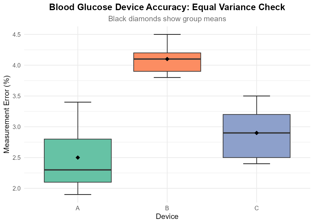
Fig. 12.11 Side-by-side boxplots for equal variance assessment.

Part (d): Normality check

With only n = 5 per group, formal normality assessment is limited. Visual checks:

# Faceted histograms (limited with n=5)
xbar <- tapply(glucose$Error, glucose$Device, mean)
s <- tapply(glucose$Error, glucose$Device, sd)

glucose$normal.density <- mapply(function(val, dev) {
  dnorm(val, mean = xbar[dev], sd = s[dev])
}, glucose$Error, glucose$Device)

ggplot(glucose, aes(x = Error)) +
  geom_histogram(aes(y = after_stat(density)),
                 bins = 4, fill = "grey", col = "black") +
  geom_density(col = "red", linewidth = 1) +
  geom_line(aes(y = normal.density), col = "blue", linewidth = 1) +
  facet_wrap(~ Device) +
  ggtitle("Normality Check: Histograms by Device") +
  xlab("Measurement Error (%)") +
  ylab("Density") +
  theme_minimal()

# Faceted QQ-plots
ggplot(glucose, aes(sample = Error)) +
  stat_qq() +
  stat_qq_line(color = "red", linewidth = 1) +
  facet_wrap(~ Device) +
  ggtitle("Normality Check: QQ-Plots by Device") +
  xlab("Theoretical Quantiles") +
  ylab("Sample Quantiles") +
  theme_minimal()

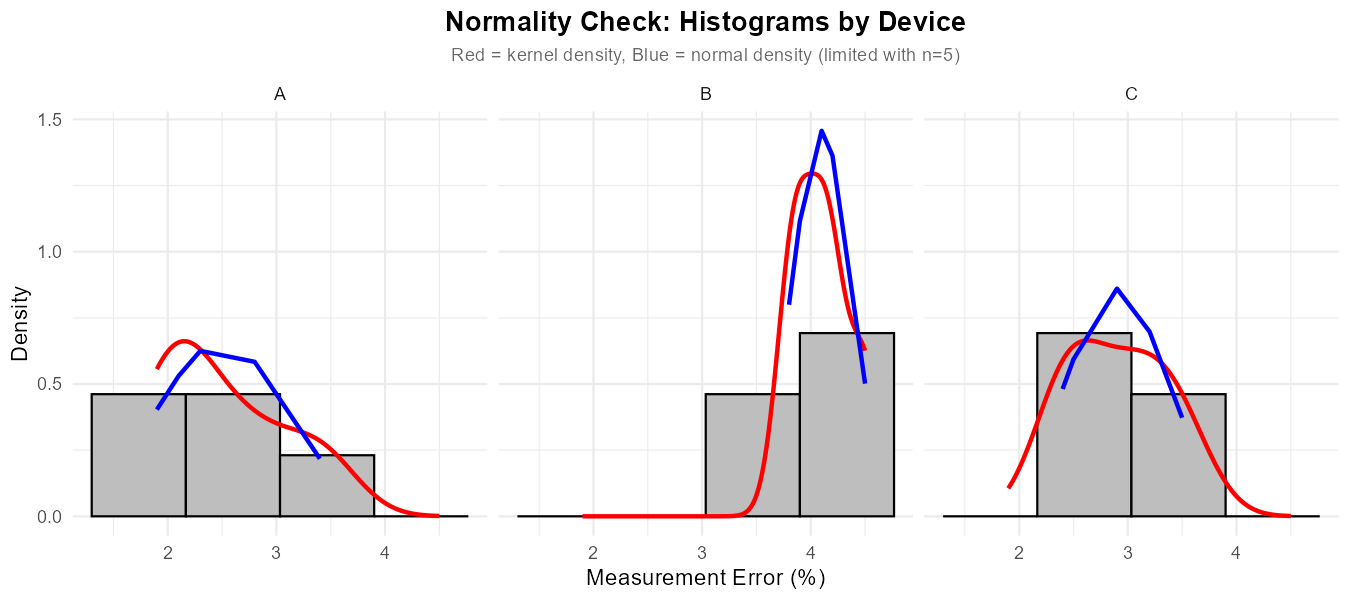
Fig. 12.12 Faceted histograms with kernel density (red) and normal overlay (blue).

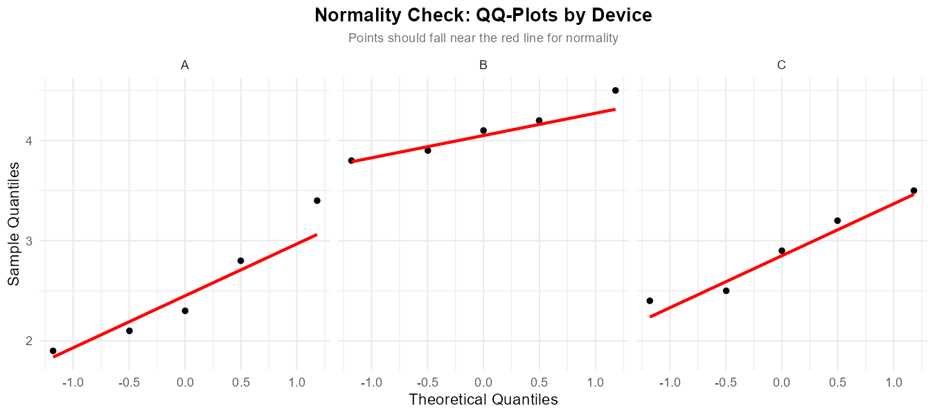
Fig. 12.13 Faceted QQ-plots for normality assessment.

Note: With only 5 observations per group, histograms are very rough and QQ-plots have few points. For such small samples, normality is difficult to assess visually. We generally rely on the robustness of ANOVA to moderate non-normality when sample sizes are equal.

Part (e): Sums of Squares

SSA (between groups):

\[\text{SSA} = 5(2.50 - 3.167)^2 + 5(4.10 - 3.167)^2 + 5(2.90 - 3.167)^2\]

\[= 5(0.445) + 5(0.869) + 5(0.071) = 2.22 + 4.35 + 0.36 = 6.93\]

SSE (within groups):

\[\text{SSE} = (5-1)(0.365) + (5-1)(0.075) + (5-1)(0.215) = 1.46 + 0.30 + 0.86 = 2.62\]

SST (total):

\[\text{SST} = \text{SSA} + \text{SSE} = 6.93 + 2.62 = 9.55\]

Part (f): ANOVA Table

Source	df	SS	MS
Device	2	6.93	3.47
Error	12	2.62	0.22
Total	14	9.55

R verification:

A <- c(2.1, 3.4, 2.8, 1.9, 2.3)
B <- c(4.2, 3.8, 4.5, 3.9, 4.1)
C <- c(2.9, 3.2, 2.5, 3.5, 2.4)

xbar <- c(mean(A), mean(B), mean(C))  # 2.50, 4.10, 2.90
grand_mean <- mean(c(A, B, C))  # 3.167
s <- c(sd(A), sd(B), sd(C))  # 0.604, 0.274, 0.464

max(s)/min(s)  # 2.20 - borderline

n <- c(5, 5, 5)
SSA <- sum(n * (xbar - grand_mean)^2)  # 6.93
SSE <- sum((n-1) * s^2)  # 2.62
SST <- SSA + SSE  # 9.55

MSA <- SSA / 2  # 3.47
MSE <- SSE / 12  # 0.22

---

Exercise 9: Conceptual Understanding of Variability Sources

Answer each question with a brief explanation.

1. Under the null hypothesis \(H_0: \mu_1 = \mu_2 = ... = \mu_k\), what should the expected value of MSA be approximately equal to? Why?

2. Is the expected value of MSE affected by whether \(H_0\) is true or false? Explain.

3. A researcher obtains MSA = 15.2 and MSE = 48.7. What does this suggest about the null hypothesis?

4. Can SSA ever be larger than SST? Why or why not?

5. If all observations in a dataset were identical (e.g., all equal to 50), what would SST, SSA, and SSE each equal?

Solution

Part (a): Expected value of MSA under H₀

Under \(H_0\), \(E(\text{MSA}) \approx \sigma^2\).

When all population means are equal, the only source of variation in group sample means is random sampling variability. The group means \(\bar{X}_{i.}\) will vary around the common population mean, and this variation is determined by \(\sigma^2\). Thus, MSA estimates \(\sigma^2\) when H₀ is true.

Part (b): E(MSE) and H₀

No, E(MSE) = σ² regardless of whether H₀ is true or false.

MSE measures variability within groups—how observations deviate from their respective group means. This within-group variability is determined by σ² (assuming equal variances) and is not affected by whether the population means differ. MSE is always an unbiased estimator of σ².

Part (c): MSA = 15.2, MSE = 48.7

This suggests there is no evidence against H₀.

The ratio F = MSA/MSE = 15.2/48.7 = 0.31, which is less than 1. This indicates that the between-group variability is actually smaller than the within-group variability—the opposite of what we’d expect if the means truly differed. We would fail to reject H₀.

Part (d): Can SSA > SST?

No, SSA can never exceed SST.

By the fundamental identity: SST = SSA + SSE

Since SSE ≥ 0 (it’s a sum of squared deviations), we must have SSA ≤ SST. Equality (SSA = SST) occurs only when SSE = 0, which happens only if all observations within each group are identical to their group mean.

Part (e): All observations identical

If all observations equal 50:

• All group means equal 50

• The grand mean equals 50

• \(\text{SST} = \sum\sum(x_{ij} - 50)^2 = 0\)

• \(\text{SSA} = \sum n_i(50 - 50)^2 = 0\)

• \(\text{SSE} = \sum\sum(x_{ij} - 50)^2 = 0\)

All sums of squares equal zero because there is no variability whatsoever.

---

12.2.7. Additional Practice Problems

True/False Questions (1 point each)

1. SSE measures the variability in the data that can be explained by group membership.

   Ⓣ or Ⓕ

2. If SSA = 500 and SST = 1200, then SSE = 700.

   Ⓣ or Ⓕ

3. MSE is an unbiased estimator of σ² only when the null hypothesis is true.

   Ⓣ or Ⓕ

4. The degrees of freedom for SST always equals the sum of df_A and df_E.

   Ⓣ or Ⓕ

5. A small value of SSA relative to SSE suggests that group means differ substantially.

   Ⓣ or Ⓕ

Multiple Choice Questions (2 points each)

6. In an ANOVA with k = 4 groups and n = 48 total observations, df_E equals:

   Ⓐ 3

   Ⓑ 44

   Ⓒ 47

   Ⓓ 48

7. The formula \(\text{SSE} = \sum_{i=1}^{k}(n_i - 1)s_i^2\) requires which assumption?

   Ⓐ Equal sample sizes

   Ⓑ Normal populations

   Ⓒ Equal population variances

   Ⓓ None—it’s always valid

8. If MSA = 250 and df_A = 5, then SSA equals:

   Ⓐ 50

   Ⓑ 255

   Ⓒ 1250

   Ⓓ 245

9. Which quantity can be used to estimate the common population standard deviation σ?

   Ⓐ √MSA

   Ⓑ √MSE

   Ⓒ √SST

   Ⓓ SSE/SST

10. In the ANOVA model \(X_{ij} = \mu_i + \varepsilon_{ij}\), the term \(\varepsilon_{ij}\) represents:

    Ⓐ The population mean for group i

    Ⓑ The random error for observation j in group i

    Ⓒ The between-group variability

    Ⓓ The grand mean

11. If all group sample means were identical (\(\bar{x}_{1.} = \bar{x}_{2.} = ... = \bar{x}_{k.}\)), what would SSA equal?

    Ⓐ SST

    Ⓑ SSE

    Ⓒ 0

    Ⓓ Cannot determine

Answers to Practice Problems

True/False Answers:

1. False — SSE measures within-group variability (unexplained by group membership). SSA measures between-group variability (explained by groups).

2. True — From SST = SSA + SSE: SSE = 1200 - 500 = 700.

3. False — MSE is an unbiased estimator of σ² regardless of whether H₀ is true, as long as the equal variance assumption holds.

4. True — df_T = df_A + df_E is part of the fundamental ANOVA identity.

5. False — Small SSA relative to SSE suggests group means are similar (little between-group variation). Large SSA suggests means differ.

Multiple Choice Answers:

6. Ⓑ — df_E = n - k = 48 - 4 = 44

7. Ⓓ — The formula is always valid; it’s a mathematical identity for computing SSE from group statistics.

8. Ⓒ — SSA = MSA × df_A = 250 × 5 = 1250

9. Ⓑ — σ̂ = √MSE is the standard estimator for the common standard deviation.

10. Ⓑ — ε_ij represents the random error component for observation j in group i.

11. Ⓒ — If all group means equal the grand mean, then (x̄_i. - x̄_..)² = 0 for all i, so SSA = 0.