Slides 📊
4.4. Law of Total Probability and Bayes’ Rule
When we make decisions under uncertainty, we often need to revise our probability assessments as new information emerges. Medical diagnoses, legal judgments, and even everyday decisions typically involve updating our beliefs based on partial evidence. In this chapter, we’ll develop the foundational principles of Bayes’ Rule, which provides a framework for this fundamental process of learning from evidence.
Road Map 🧭
Define partitions of the sample space and derive the law of partitions.
Build upon this to establish the law of total probability.
Develop Bayes’ rule for inverting conditional probabilities.
4.4.1. Law of Partitions
What is a Partition?
A collection of events \(\{A_1, A_2, \cdots, A_n\}\) forms a partition of the sample space \(\Omega\) if the following two conditions are satisfied.
The events are mutually exclusive:
\[A_i \cap A_j = \emptyset \text{ for all } i \neq j.\]The events are exhaustive:
\[A_1 \cup A_2 \cup \cdots \cup A_n = \Omega.\]
In other words, a partition divides the sample space into non-overlapping pieces that, when combined, reconstruct the entire space. You can think of a partition as pizza slices—each slice represents an event, the slices do not overlap, and together they make up a whole pizza.
The law of partitions provides a way to calculate the probability of a new event by examining how it intersects with each part of a partition.
Note ✏️
The simplest example of a partition consists of just two events: any event \(A\) and its complement \(A'\). These two events are
mutually exclusive because \(A \cap A' = \emptyset\), and
exhaustive because together they cover the entire sample space (\(A \cup A' = \Omega\)).
Law of Partitions
If \(\{A_1, A_2, \cdots, A_n\}\) forms a partition of the sample space \(\Omega\), then for any event \(B\) in the same sample space:
What Does It Say?
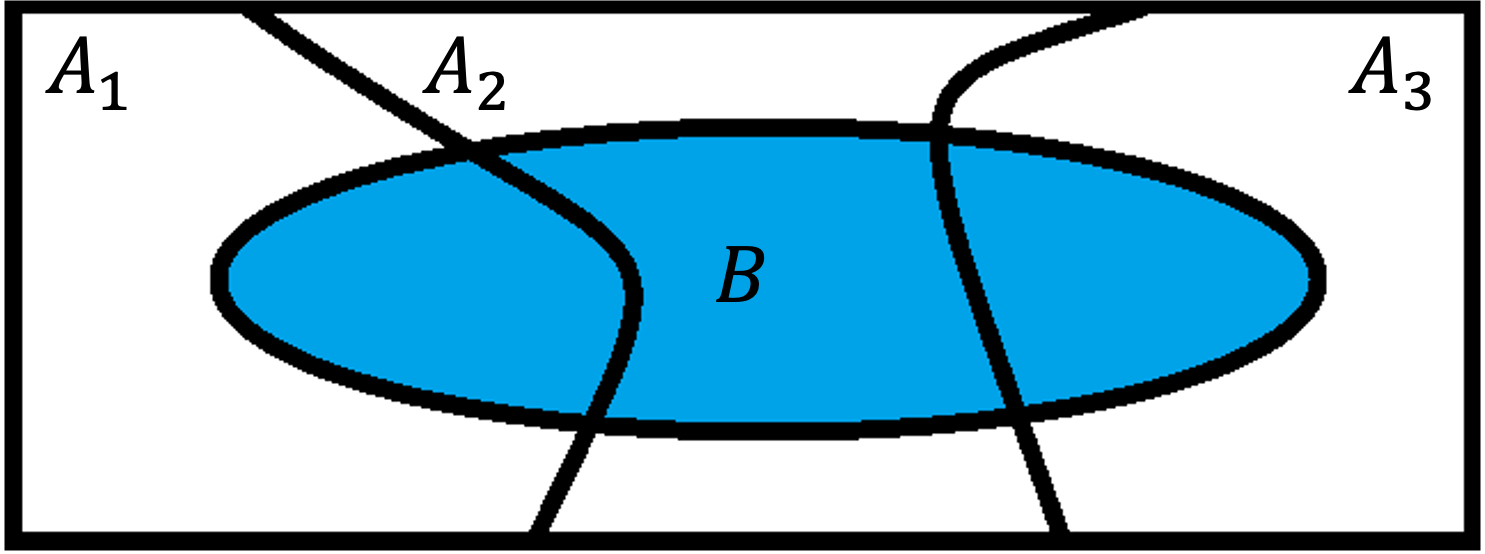
Fig. 4.17 Law of partitions
Take a partition that consists of three events as in Fig. 4.17. Then, the Law of Partitions can be expanded to
The left-hand side of the equation points to the relative area of the whole blue region, while each term on the right-hand side points to the relative area of a smaller piece created by the overlap of \(B\) with one of the events in the partition.
The core message of the Law of Partitions is quite simple; the probability of the whole is equal to the sum of the probabilities of its parts.
4.4.2. Law of Total Probability
The Law of Total Probability takes the Law of Partitions one step further by rewriting the intersection probabilities using the general multiplication rule.
Reminder🔎: The General Multiplication Rule
For any two events \(C\) and \(D\), \(P(C \cap D) = P(C|D) P(D) = P(D|C) P(C).\)
Statement
If \(\{A_1, A_2, \cdots, A_n\}\) forms a partition of the sample space \(\Omega\), then for any event \(B \subseteq \Omega\),
What Does It Say?
Fig. 4.18 Law of Total Probability
Let us continue to use the simple three-event partition. The Law of Total Probability says
The Law of Total Probability now expresses the probability of event \(B\) as a weighted average of conditional probabilities. Each weight \(P(A_i)\) represents the probability of a particular part in the sample space, and each conditional probability \(P(B|A_i)\) represents the likelihood of \(B\) given that we are in that part.
The Law of Total Probability on a Tree diagram
Recall that in a tree diagram, the set of branches extending from the same node must represent all possible outcomes given the preceding path. This requirement is, in fact, another way of saying that these branches must form a partition. As a result, a tree diagram provides an ideal setting for applying the Law of Total Probability.
Computing a single-stage probability \(P(B)\) using the Law of Total Probability is equivalent to
finding the path probabilties of all paths involving \(B\),
then summing the probabilities.
Try writing these steps down in mathematical notation and confirm that they are identical to applying the Law of Total Probability directly.
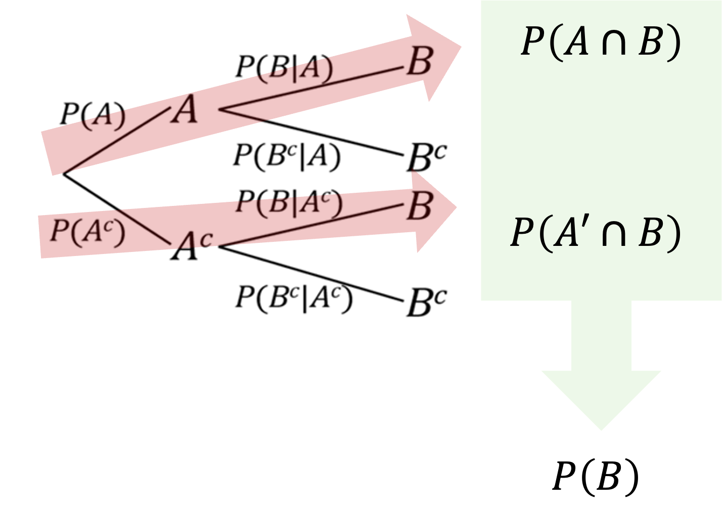
Fig. 4.19 Using the Law of Total Probability with a tree diagram
Example💡: The Law of Partitions and the Law of Total Probability
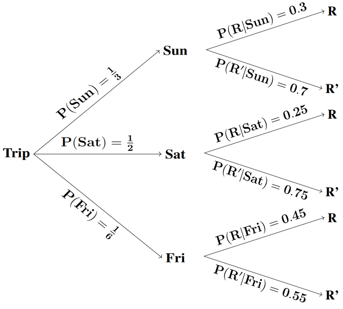
Fig. 4.20 Tree diagram for the Indianapolis problem
Recall the Indianapolis example from the previous section. In this problem, what is the probability that it rains?
First equality uses the Law of Partitions. The second equality uses the Law of Total Probability.
Confirm that the mathematical steps and the final outcome are identical when the tree diagram is used.
4.4.3. Bayes’ Rule
Bayes’ rule allows us to invert conditional probabilities. That is, it allows us to compute \(P(A|B)\) from our knowledge of \(P(B|A).\)
Statement
If \(\{A_1, A_2, \cdots, A_n\}\) forms a partition of the sample space \(\Omega\), and \(B\) is an event with \(P(B) > 0\), then for any \(i=1,2,\cdots,n\),
For the simplified case of a three-event partition, Bayes’ rule for \(P(A_1|B)\) is:
Graphically, this equation represents the ratio of the area of the first blue piece (\(A_1 \cap B\)) over the whole area of \(B\) in Fig. 4.21.
Fig. 4.21 Visual aid for Bayes’ Rule
Derivation of Bayes’ Rule
First equality: definition of conditional probability
Second equality: Law of Total Probability for the denominator
Third equality: the general multiplication rule for the numerator
Example💡: Bayes’ Rule
The Indianapolis example is continued. Knowing that it didn’t rain on the day Glen and Jia went to Indianapolis, find the probability that this was Friday.
\(P(R')\) can be computed directly using the tree diagram or the Law of Total Probability. However, using the complement rule is more convenient since we already have \(P(R)\) from the previous part.
4.4.4. Understanding the Bayesian Approach to Probability through Bayes’ Rule
Bayes’ rule forms the foundation of the Bayesian approach to probability, which interprets probabilities as degrees of belief that can be updated as new evidence emerges.
Each component of Bayes’ rule has a Bayesian interpretation:
\(P(A_i)\): the prior probability
The initial assessment of the probability of event \(A_1\)
\(P(B|A_i)\): the likelihood
The probability of observing a new evidence \(B\) given that \(A_1\) holds. This measures how consistent the evidence is with \(A_i\).
\(P(A_i|B)\): the posterior probability
The updated probability of \(A_i\) accounting for the evidence \(B\).
\(P(B)\): the normalizing constant
Once the evidence \(B\) is observed, the sample space shrinks to only the region that would have made \(B\) possible. Computing a posterior probability involves a step where we divide probabilities by \(P(B)\), the size of a new whole (see the second step of deriving Bayes rule).
As we gather more evidence, we can repeatedly apply Bayes’ rule, using the posterior probability from one calculation as the prior probability for the next. This iterative process allows our probability assessments to continuously improve as we incorporate new information.
Comprehensive Example💡: Medical Testing
Consider a disease that affects a small percentage of the population and a diagnostic test used to detect it.
Let \(D\) be the event that a person has the disease.
Let \(+\): be the event that the test gives a positive result.
Define \(D'\) and \(-\) as the complements of \(D\) and \(+\), respectively
Given these events, we can identify:
\(P(D)\): The prevalence of the disease in the population (prior probability)
\(P(+|D)\): The sensitivity of the test (true positive rate)
\(P(+|D')\): The false positive rate (1 - specificity)
What doctors and patients typically want to know is \(P(D|+)\), the probability that a person has the disease given a positive test result. This posterior probability can be calculated using Bayes’ rule:
Suppose a disease affects 1% of the population, the test has a sensitivity of 95%, and a specificity of 90%. What is the probability that someone with a positive test result actually has the disease?
Step 1: Write the building blocks in mathematical notation
\(P(D) = 0.01\)
\(P(+|D) = 0.95\)
\(P(+|D') = 1-P(-|D') = 1 - 0.9 = 0.1\)
Step 2: Compute the posterior probability
Despite the test being quite accurate (95% sensitivity, 90% specificity), the probability that a positive result indicates disease is less than 9%. This illustrates the importance of considering the base rate (prior probability) when interpreting test results, especially for rare conditions. Even a very accurate test will generate many false positives when applied to a population where the condition is uncommon.
Also try solving this problem using a tree diagram, and confirm that the results are consistent.
4.4.5. Bringing It All Together
Key Takeaways 📝
The Law of Partitions decomposes the probability of an event across a partition.
The Law of Total Probability expresses an event’s probability as a weighted average of conditional probabilities.
Bayes’ rule lets us calculate “inverse” conditional probabilities.
Tree diagrams serve as an assisting tool for the three rules above.
Bayes’ rule forms the foundation of the Bayesian approach to probability.
4.4.6. Exercises
These exercises develop your skills in applying the Law of Total Probability and Bayes’ Rule to solve multi-stage probability problems.
Exercise 1: Identifying Partitions
For each scenario, determine whether the given collection of events forms a valid partition of the sample space. If not, explain which condition (mutually exclusive or exhaustive) is violated.
Sample space: All students in a class. Events: \(A_1\) = “freshman”, \(A_2\) = “sophomore”, \(A_3\) = “junior”, \(A_4\) = “senior”
Sample space: All possible outcomes when rolling a six-sided die. Events: \(B_1\) = “even number”, \(B_2\) = “odd number”
Sample space: All employees at a company. Events: \(C_1\) = “works in engineering”, \(C_2\) = “works in marketing”, \(C_3\) = “has been with the company more than 5 years”
Sample space: All real numbers from 0 to 100. Events: \(D_1 = [0, 50)\), \(D_2 = [50, 100]\)
Sample space: Results of a software test. Events: \(E_1\) = “test passes”, \(E_2\) = “test fails with minor error”
Solution
Part (a): Valid Partition ✓
Mutually exclusive: A student can only be in one class year at a time. ✓
Exhaustive: Every student must be a freshman, sophomore, junior, or senior. ✓
Part (b): Valid Partition ✓
Mutually exclusive: A number cannot be both even and odd. ✓
Exhaustive: Every integer is either even or odd. ✓
Note: \(B_1\) and \(B_2\) form the simplest partition — an event and its complement.
Part (c): NOT a Valid Partition ✗
Mutually exclusive: VIOLATED. An engineer could also have been with the company more than 5 years. The events overlap.
Exhaustive: VIOLATED. An employee in finance with 2 years tenure wouldn’t be in any of these events.
Part (d): Valid Partition ✓
Mutually exclusive: \([0, 50)\) and \([50, 100]\) don’t overlap (50 is only in the second set). ✓
Exhaustive: Together they cover all numbers from 0 to 100. ✓
Part (e): NOT a Valid Partition ✗
Mutually exclusive: These could be mutually exclusive if properly defined. ✓
Exhaustive: VIOLATED. What about “test fails with major error” or “test crashes”? The events don’t cover all possible outcomes.
Exercise 2: Law of Total Probability
A data center has three server clusters that handle incoming requests:
Cluster A handles 50% of all requests
Cluster B handles 30% of all requests
Cluster C handles 20% of all requests
Due to different hardware and configurations, the probability of a request being processed successfully varies by cluster:
Cluster A: 99% success rate
Cluster B: 97% success rate
Cluster C: 95% success rate
Define appropriate events and write out the given information using probability notation.
Use the Law of Total Probability to find the overall probability that a randomly selected request is processed successfully.
What is the probability that a randomly selected request fails?
Draw a tree diagram representing this situation and verify your answer to part (b).
Solution
Part (a): Define Events and Notation
Let:
\(A\) = request handled by Cluster A
\(B\) = request handled by Cluster B
\(C\) = request handled by Cluster C
\(S\) = request processed successfully
Given information:
\(P(A) = 0.50\), \(P(B) = 0.30\), \(P(C) = 0.20\)
\(P(S|A) = 0.99\), \(P(S|B) = 0.97\), \(P(S|C) = 0.95\)
Note: \(\{A, B, C\}\) forms a partition since clusters are mutually exclusive and exhaustive.
Part (b): Law of Total Probability
The overall success rate is 97.6%.
Part (c): Probability of Failure
Using the complement rule:
The overall failure rate is 2.4%.
Part (d): Tree Diagram
             [Start]
            /   |   \
     0.50  /    |0.30 \  0.20
          /     |      \
        [A]    [B]     [C]
       / \    /  \    /  \
0.99  /   \  /    \  /    \ 0.05
     /  0.01\0.97 0.03\0.95  \
   [S]  [S'] [S] [S'] [S]  [S']
    |     |   |    |   |     |
 0.495  0.005 0.291 0.009 0.190 0.010
Sum of success paths: \(0.495 + 0.291 + 0.190 = 0.976\) ✓
Exercise 3: Bayes’ Rule — Manufacturing
An electronics manufacturer sources microprocessors from three suppliers:
Supplier X provides 40% of processors with a 2% defect rate
Supplier Y provides 35% of processors with a 3% defect rate
Supplier Z provides 25% of processors with a 5% defect rate
A randomly selected processor is found to be defective.
What is the probability that it came from Supplier X?
What is the probability that it came from Supplier Y?
What is the probability that it came from Supplier Z?
Verify that your answers to parts (a), (b), and (c) sum to 1.
Which supplier is most likely responsible for a defective processor? Is this the same as the supplier with the highest defect rate?
Solution
Setup:
Let \(X, Y, Z\) denote the suppliers and \(D\) = “processor is defective.”
Given:
\(P(X) = 0.40\), \(P(D|X) = 0.02\)
\(P(Y) = 0.35\), \(P(D|Y) = 0.03\)
\(P(Z) = 0.25\), \(P(D|Z) = 0.05\)
First, find P(D) using Law of Total Probability:
Part (a): P(X|D)
Part (b): P(Y|D)
Part (c): P(Z|D)
Part (d): Verification
\(P(X|D) + P(Y|D) + P(Z|D) = 0.2581 + 0.3387 + 0.4032 = 1.0000\) ✓
This must be true since \(\{X, Y, Z\}\) partitions the sample space.
Part (e): Interpretation
Supplier Z is most likely responsible for a defective processor (40.32% probability).
This is the same as the supplier with the highest defect rate (5%). However, it’s not always the case! If Supplier Z only provided 5% of processors instead of 25%, the answer would change. Bayes’ Rule accounts for both:
The defect rate (likelihood)
The proportion of supply (prior)
Exercise 4: Bayes’ Rule — Diagnostic Testing
A new screening test for a rare genetic condition is being evaluated. The condition affects 1 in 500 people in the general population. Clinical trials show:
Sensitivity (true positive rate): 98% — P(+|Disease) = 0.98
Specificity (true negative rate): 96% — P(−|No Disease) = 0.96
Calculate the probability that a person who tests positive actually has the condition. (This is called the positive predictive value.)
Calculate the probability that a person who tests negative does not have the condition. (This is called the negative predictive value.)
If the test is used to screen 10,000 people, approximately how many will test positive? Of those, how many actually have the condition?
Why is the positive predictive value so much lower than the sensitivity, even though both the sensitivity and specificity are quite high?
Solution
Setup:
\(P(D) = 1/500 = 0.002\) (prevalence)
\(P(D') = 0.998\)
\(P(+|D) = 0.98\) (sensitivity)
\(P(-|D') = 0.96\) (specificity)
\(P(+|D') = 1 - 0.96 = 0.04\) (false positive rate)
Part (a): Positive Predictive Value P(D|+)
First, find P(+) using Law of Total Probability:
Now apply Bayes’ Rule:
Positive Predictive Value ≈ 4.68%
Part (b): Negative Predictive Value P(D’|−)
First, find P(−):
Find \(P(-|D) = 1 - P(+|D) = 1 - 0.98 = 0.02\) (false negative rate)
Negative Predictive Value ≈ 99.996%
Part (c): Screening 10,000 People
Expected positive tests: \(10,000 \times P(+) = 10,000 \times 0.04188 \approx 419\) people
Of those with positive tests, expected true positives:
People with disease: \(10,000 \times 0.002 = 20\)
True positives (disease AND positive): \(20 \times 0.98 \approx 20\) people
So approximately 419 test positive, but only about 20 actually have the condition.
Part (d): Why is PPV So Low?
Even though the test has high sensitivity (98%) and specificity (96%), the base rate of the disease is very low (0.2%).
When the disease is rare:
The number of true positives is small (98% of a small number)
The number of false positives is much larger (4% of a very large number)
With 10,000 people:
True positives: ~20 (from the 20 people with disease)
False positives: ~399 (4% of the 9,980 healthy people)
Total positives: ~419, but only ~20 are real!
This is the base rate fallacy — people often overestimate PPV when the condition is rare.
Exercise 5: Multi-Stage Problem with Tree Diagram
A delivery company has two distribution centers (DC1 and DC2) that ship packages to customers. DC1 handles 60% of packages and DC2 handles 40%.
Packages from DC1 are shipped via Ground (80%) or Express (20%)
Packages from DC2 are shipped via Ground (50%) or Express (50%)
The on-time delivery rates are:
DC1 Ground: 92% on-time
DC1 Express: 98% on-time
DC2 Ground: 88% on-time
DC2 Express: 99% on-time
Draw a complete three-stage tree diagram for this problem.
What is the probability that a randomly selected package is delivered on time?
Given that a package was delivered late, what is the probability it came from DC1?
Given that a package was delivered late, what is the probability it was shipped via Ground?
Solution
Part (a): Tree Diagram
                  [Start]
                 /       \
          0.60  /         \ 0.40
               /           \
            [DC1]         [DC2]
           /    \         /    \
     0.80 /      \0.20   /0.50  \ 0.50
         /        \     /        \
       [G]       [E]  [G]        [E]
      /  \      /  \  /  \      /   \
0.92 / \0.08 0.98\0.02 0.88\0.12 0.99\ 0.01
    /   \    /   \   /    \   /     \
  [OT] [L] [OT] [L] [OT]  [L] [OT]  [L]
Path probabilities:
DC1, Ground, On-Time: 0.60 × 0.80 × 0.92 = 0.4416
DC1, Ground, Late: 0.60 × 0.80 × 0.08 = 0.0384
DC1, Express, On-Time: 0.60 × 0.20 × 0.98 = 0.1176
DC1, Express, Late: 0.60 × 0.20 × 0.02 = 0.0024
DC2, Ground, On-Time: 0.40 × 0.50 × 0.88 = 0.1760
DC2, Ground, Late: 0.40 × 0.50 × 0.12 = 0.0240
DC2, Express, On-Time: 0.40 × 0.50 × 0.99 = 0.1980
DC2, Express, Late: 0.40 × 0.50 × 0.01 = 0.0020
Part (b): P(On-Time)
Sum all on-time paths:
93.32% of packages are delivered on time.
Part (c): P(DC1|Late)
First, find P(Late):
P(DC1 ∩ Late) = P(DC1, Ground, Late) + P(DC1, Express, Late) = 0.0384 + 0.0024 = 0.0408
Given a late package, there’s about a 61.08% chance it came from DC1.
Part (d): P(Ground|Late)
P(Ground ∩ Late) = P(DC1, Ground, Late) + P(DC2, Ground, Late) = 0.0384 + 0.0240 = 0.0624
Given a late package, there’s about a 93.41% chance it was shipped via Ground.
Exercise 6: Prior and Posterior Probabilities
A machine learning model classifies emails as “spam” or “not spam.” Before seeing any features of an email:
Prior probability: 30% of incoming emails are spam
The model uses the presence of the word “FREE” as a feature:
P(“FREE” appears | Spam) = 0.60
P(“FREE” appears | Not Spam) = 0.10
An email arrives containing the word “FREE.” What is the posterior probability that it is spam?
An email arrives that does NOT contain the word “FREE.” What is the posterior probability that it is spam?
Compare the prior and posterior probabilities. How much does observing “FREE” change our belief about whether the email is spam?
The model now also considers the presence of “URGENT.” Given that an email is spam: - P(“URGENT” | Spam) = 0.40
Given that an email is not spam: - P(“URGENT” | Not Spam) = 0.05
If an email contains BOTH “FREE” and “URGENT” (assume these are conditionally independent given spam status), what is the posterior probability it is spam?
Solution
Setup:
\(P(S) = 0.30\) (prior — email is spam)
\(P(S') = 0.70\) (prior — email is not spam)
\(P(F|S) = 0.60\) (“FREE” given spam)
\(P(F|S') = 0.10\) (“FREE” given not spam)
Part (a): P(Spam | “FREE” appears)
First, find P(F) using Law of Total Probability:
Apply Bayes’ Rule:
Posterior probability of spam given “FREE”: 72%
Part (b): P(Spam | “FREE” does NOT appear)
First, find P(F’) = 1 − 0.25 = 0.75
Find \(P(F'|S) = 1 - P(F|S) = 1 - 0.60 = 0.40\)
Posterior probability of spam given NO “FREE”: 16%
Part (c): Comparison
Prior P(Spam) = 0.30 (before seeing any features)
Posterior P(Spam | “FREE”) = 0.72 (increased dramatically)
Posterior P(Spam | no “FREE”) = 0.16 (decreased)
Observing “FREE” increases our belief that the email is spam from 30% to 72% — more than doubling it. The absence of “FREE” decreases our belief to 16% — nearly halving it.
The word “FREE” is a strong indicator because it’s 6 times more likely to appear in spam (60%) than in legitimate email (10%).
Part (d): P(Spam | “FREE” AND “URGENT”)
With conditional independence, we can update sequentially. Start with the posterior from part (a) as the new prior:
New prior: P(S) = 0.72 (given “FREE”)
P(U|S) = 0.40
P(U|S’) = 0.05
Find P(U | already observed “FREE”):
Apply Bayes’ Rule:
Posterior probability of spam given BOTH “FREE” and “URGENT”: ~95.4%
Each piece of evidence updates our belief. Starting from 30%, “FREE” brings us to 72%, and “URGENT” further increases it to 95.4%.
4.4.7. Additional Practice Problems
True/False Questions (1 point each)
A partition of a sample space must consist of at least three events.
Ⓣ or Ⓕ
The Law of Total Probability requires that the conditioning events form a partition.
Ⓣ or Ⓕ
Bayes’ Rule allows us to compute \(P(A|B)\) when we know \(P(B|A)\).
Ⓣ or Ⓕ
In Bayes’ Rule, the denominator is computed using the Law of Total Probability.
Ⓣ or Ⓕ
If a medical test has high sensitivity (99%), then a positive result means the patient almost certainly has the disease.
Ⓣ or Ⓕ
When using Bayes’ Rule, the posterior probabilities for all events in the partition must sum to 1.
Ⓣ or Ⓕ
Multiple Choice Questions (2 points each)
Factory A produces 60% of a product with 2% defective. Factory B produces 40% with 5% defective. What is P(defective)?
Ⓐ 0.012
Ⓑ 0.020
Ⓒ 0.032
Ⓓ 0.035
Using the information from Question 7, if a product is defective, what is P(from Factory A)?
Ⓐ 0.375
Ⓑ 0.400
Ⓒ 0.600
Ⓓ 0.625
A disease affects 2% of the population. A test has 95% sensitivity and 90% specificity. What is P(Disease | Positive)?
Ⓐ About 16%
Ⓑ About 50%
Ⓒ About 90%
Ⓓ About 95%
In the Bayesian framework, which term describes \(P(A_i)\) in Bayes’ Rule?
Ⓐ Likelihood
Ⓑ Posterior probability
Ⓒ Prior probability
Ⓓ Normalizing constant
Answers to Practice Problems
True/False Answers:
False — The simplest partition consists of just two events: an event A and its complement A’.
True — The Law of Total Probability requires that the events \(\{A_1, A_2, \ldots, A_n\}\) be mutually exclusive and exhaustive (i.e., form a partition).
True — This is exactly what Bayes’ Rule does: it “inverts” conditional probabilities.
True — The denominator \(\sum P(B|A_i)P(A_i)\) is the Law of Total Probability applied to find P(B).
False — High sensitivity means the test correctly identifies most people with the disease. But if the disease is rare, most positive results may still be false positives (low positive predictive value).
True — Since the partition events cover the entire sample space, the posterior probabilities must sum to 1: \(\sum P(A_i|B) = 1\).
Multiple Choice Answers:
Ⓒ — P(D) = P(D|A)P(A) + P(D|B)P(B) = (0.02)(0.60) + (0.05)(0.40) = 0.012 + 0.020 = 0.032
Ⓐ — P(A|D) = P(D|A)P(A) / P(D) = (0.02)(0.60) / 0.032 = 0.012 / 0.032 = 0.375
Ⓐ — P(+) = (0.95)(0.02) + (0.10)(0.98) = 0.019 + 0.098 = 0.117. P(D|+) = 0.019/0.117 ≈ 0.162 ≈ 16%
Ⓒ — \(P(A_i)\) is the prior probability — our initial belief before observing evidence B.