Slides 📊
11.2. Independent Two-Sample Analysis When Population Variances Are Known
We now develop the mathematical foundation for comparing the means of two independent populations, assuming that the population variances are known. The simplifying assumption will be lifted in later lessons when we discuss more realistic scenarios.
Road Map 🧭
List the three key assumptions required for the construction of independent two-sample inference methods.
Construct hypothesis tests and confidence regions for the difference in the means of two independent populations. Identify the common underlying principles with one-sample inference.
11.2.1. The Assumptions
The validity of independent two-sample procedures rests on three fundamental assumptions that extend the single-sample framework to comparisons. These assumptions must be carefully verified before applying the methods.
Assumption 1: SRS from Each Population
The random variables \(X_{A1}, X_{A2}, \ldots, X_{An_A}\) form an independent and identically distributed (iid) sample from Population A. Similarly, the random variables \(X_{B1}, X_{B2}, \ldots, X_{Bn_B}\) constitute an iid sample from Population B.
Assumption 2: Independence Between Populations
The observations from one population are independent of those from the other population. Formally, \(X_{Ai}\) is independent of \(X_{Bj}\) for all possible pairs of indices \(i \in \{1, 2, \ldots, n_A\}\) and \(j \in \{1, 2, \ldots, n_B\}\).
Assumption 3: Normality of Sampling Distributions
For each population, either the population distribution is normal, or the sample size is large enough for the CLT to hold.
11.2.2. The Parameter of Interest and Its Point Estimator
The Target Parameter
Recall that our primary interest lies not in the individual population means \(\mu_A\) and \(\mu_B\), but rather in their difference. Our parameter of interest is:
We conceptualize this difference as a single parameter that captures the essence of the comparison we wish to make. Its sign and magnitude indicate the direction and size of any systematic difference between the populations.
The Point Estimator
Since we know that \(\bar{X}_A\) and \(\bar{X}_B\) are unbiased estimators of their respective population means \(\mu_A\) and \(\mu_B\), the natural point estimator for \(\theta\) is:
11.2.3. Theoretical Properties of the Point Estimator
As a result of Assumptions 1 and 3, the sampling distributions of the two sample means are:
Furthermore, the two random variables are independent since their building blocks are independent according to Assumption 2. We establish the theoretical properties of the difference estimator \(\bar{X}_A - \bar{X}_B\) starting from this baseline.
Unbiasedness
The difference in sample means is an unbiased estimator of the difference in population means. To establish this formally:
Therefore, the bias of the estimator is:
Variance of the Estimator
The variance of \(\bar{X}_A - \bar{X}_B\) depends critically on the independence assumption between populations. Recall that for two independent random variables, the variance of their difference equals the sum of their individual variances:
Standard Error
The standard deviation of the estimator, or the standard error, is obtained by taking the square root of the variance:
The Sampling Distribution of the Difference Estimator
We now know the expected value and variance of the difference estimator \(\bar{X}_A - \bar{X}_B\). Additionally, since \(\bar{X}_A\) and \(\bar{X}_B\) are each normally distributed, their difference is also normally distributed. Combining these results, we establish the full sampling distribution of the difference estimator as:
Equivalently, its standardization follows the standard normal distribution:
Based on these key results, we will now build inference methods for the difference in population means.
11.2.4. Hypothesis Testing for the Difference in Means
The four-step hypothesis testing framework extends naturally to the two-sample setting, with modifications to accommodate the comparative nature.
Step 1: Parameter Identification
We must clearly identify both population means using contextually meaningful labels. Rather than generic labels like A and B, we encourage the use of descriptive terms that reflect the populations being studied.
For example, suppose we are comparing the systolic blood pressure of two patient groups after assigning one group a placebo and the other a newly developed treatment. We can define the relevant populations and their true means in the following manner:
Let \(\mu_{\text{treatment}}\) denote the true mean systolic blood pressure of patients who are treated with the new procedure.
Let \(\mu_{\text{control}}\) denote the true mean systolic blood pressure of patients who are not treated with the new medical procedure.
The parameter identification should also specify the units of measurement and provide sufficient context for interpreting the parameter and the target population within the scope of the research question.
Step 2: Hypothesis Formulation
Follow the template:
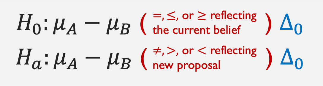
Fig. 11.2 Template for independent two-sample hypotheses
You may also refer to the details provided in Chapter 11.1.3.
Step 3: Test Statistic and \(p\)-Value
Recall the \(z\)-test statistic used in one-sample hypothesis testing:
By providing a standardized distance between the estimator and the null value, the \(z\)-test statistic measured how far the sample data is from the null assumption.
We define a new \(z\)-test statistic to serve the same purpose by replacing each one-sample component with the appropriate independent two-sample parallel:
As in the one-sample case, under the null hypothesis,
The \(p\)-value calculation therefore follows the same principles as in single-sample \(z\)-tests:
Revisiting \(p\)-Value Computation |
|
|---|---|
Upper-tailed |
\(P(Z > z_{TS})\) |
Lower-tailed |
\(P(Z < z_{TS})\) |
Two-tailed |
\(2P(Z > |z_{TS}|) = 2P(Z < -|z_{TS}|)\) |
Step 4: Decision and Conclusion
The decision rule remains unchanged from single-sample procedures:
If \(p\)-value \(\leq \alpha\), we reject \(H_0\).
If \(p\)-value \(> \alpha\), we fail to reject \(H_0\).
The conclusion template below is adapted to address the comparative nature of two-sample procedures:
“The data [does/does not] give [some/strong] support (p-value = [value]) to the claim that [statement of \(H_a\) in context about the difference in population means].”
The strength descriptors should reflect the magnitude of the \(p\)-value relative to conventional benchmarks and the significance level used in the study.
Example 💡: Shift Scheduling and Work Efficiency
A retail chain tests two different workforce scheduling systems to see which helps cashiers process more transactions per 8-hour shift. They run independent pilots on different stores:
System A: \(n_A = 25\), \(\bar{x}_A = 50\), \(\sigma_A = 10\) (known)
System B: \(n_B = 30\), \(\bar{x}_B = 45\), \(\sigma_B = 12\) (known)
Perform a hypothesis test to determine whether the true mean numbers of transactions are different at the \(\alpha = 0.05\) significance level.
Step 1: Define the parameters and target populations
Let \(\mu_A\) denote the true mean number of transactions processed by cashiers following System A. Likewise, let \(\mu_B\) be the true mean number of transactions completed by employees following System B.
Step 2: Write the hypotheses
Step 3: Compute the test statistic and p-value
This is a two-sided test, so the \(p\)-value is \(2P(Z > 1.68) \approx 0.093\).
Step 4: Decision and Conclusion
Since \(p\)-value \(= 0.093 > 0.05\), we fail to reject the null hypothesis at the 5% significance level. We do not have enough evidence to support the claim that the mean number of transactions fulfilled by cashiers are different by the scheduling system.
11.2.5. Confidence Regions for the Difference in Means
Let us begin by constructing a \(100C\%\) confidence interval. The goal is to find the margin of error (ME) such that
The Pivotal Method
We begin with the known truth:
Replace \(Z\) with the standardization of the difference estimator, or the pivotal quantity:
Through algebraic manipulation to isolate \(\mu_A - \mu_B\) in the center of the inequality, we obtain
with \(ME = z_{\alpha/2} \sqrt{\frac{\sigma^2_A}{n_A} + \frac{\sigma^2_B}{n_B}}\).
For a single experiment, therefore, the \(100C \%\) confidence interval is:
Complete Summary of Confidence Intervals and Bounds
The one-sided confidence bounds can be derived similarly. We leave the details as an exercise—use the confidence interval derivation above and Chapter 9.4 as reference.
\(100\cdot (1-\alpha) \%\) Confidence Regions for Difference in Means |
|
|---|---|
Confidence Interval |
\[(\bar{x}_A - \bar{x}_B) \pm z_{\alpha/2} \sqrt{\frac{\sigma^2_A}{n_A} + \frac{\sigma^2_B}{n_B}}\]
|
Upper Confidence Bound |
\[(\bar{x}_A - \bar{x}_B) + z_{\alpha} \sqrt{\frac{\sigma^2_A}{n_A} + \frac{\sigma^2_B}{n_B}}\]
|
Lower Confidence Bound |
\[(\bar{x}_A - \bar{x}_B) - z_{\alpha} \sqrt{\frac{\sigma^2_A}{n_A} + \frac{\sigma^2_B}{n_B}}\]
|
Note the repeated core elements. In both one-sample and two-sample cases, a confidence region is centered at the point estimate and expands in the appropriate directions by ME, computed as a product of a critical value and the standard error.
Interpreting Confidence Regions for Difference in Means
The confidence regions provide a range of plausible values for the true difference in population means; each region captures the true difference \(\mu_A - \mu_B\) with \(100(1-\alpha)\%\) confidence. Their precision depends on the confidence level, the population variances, and the sample sizes.
Example 💡: Shift Scheduling and Work Efficiency, Continued
For the experiment on two workforce scheduling systems with:
System A: \(n_A = 25\), \(\bar{x}_A = 50\), \(\sigma_A = 10\) (known)
System B: \(n_B = 30\), \(\bar{x}_B = 45\), \(\sigma_B = 12\) (known)
Compute the \(95 \%\) confidence interval for the difference of the two population means. Check if the result is consistent with the hypothesis test performed in the previous example.
Identify the components
The observed sample difference
\[\bar{x}_A - \bar{x}_B = 50 - 45 = 5\]The standard error
\[\sqrt{\frac{\sigma^2_A}{n_A} + \frac{\sigma^2_B}{n_B}} = \sqrt{\frac{10^2}{25} + \frac{12^2}{30}} \approx 2.97\]The \(z\)-critical value
qnorm(0.025, lower.tail=FALSE)
# returns 1.96
Put the parts together
The confidence interval is:
Is it consistent with the hypothesis test?
The interval contains zero, which is consistent with our failure to reject the null hypothesis of equal means.
11.2.6. Bringing It All Together
Key Takeaways 📝
Two-sample independent procedures are designed to provide statistical answers to comparative questions. They require the key assumptions that (1) each sample is an SRS of the respective population, (2) the two samples are independent from each other, (3) and the CLT holds in each sample.
The sampling distribution of the point estimator \(\bar{X}_A - \bar{X}_B\) is normal with mean \(\mu_A - \mu_B\) and variance \(\frac{\sigma^2_A}{n_A} + \frac{\sigma^2_B}{n_B}\). The addition of variances follows from the independence assumption between groups.
The construction of hypothesis tests and confidence regions follows the same core principles as in the one-sample case.
11.2.7. Exercises
Exercise 1: Assumptions for Independent Two-Sample z-Procedures
For each scenario, evaluate whether the assumptions for the independent two-sample z-procedure are satisfied. If not, explain which assumption is violated.
Comparing mean reaction times between gamers (n=50) and non-gamers (n=45). Both groups are randomly sampled, and historical studies suggest σ₁ = 25 ms and σ₂ = 30 ms.
Comparing mean heights between students who eat breakfast (n=20) and those who skip breakfast (n=18) in a single classroom. The population standard deviations are known from large national studies.
Comparing mean battery life between two phone models by testing 10 phones of each model. The manufacturer provides population standard deviations from extensive quality control testing.
Comparing mean customer wait times at two bank branches by sampling 100 customers at each location. Prior studies established σ₁ = 5 min and σ₂ = 7 min.
Solution
Assumptions Required:
SRS from each population (iid within each sample)
Independence between populations
Normality of sampling distributions (either normal populations or large n for CLT)
Population standard deviations σ₁ and σ₂ are known
Part (a): Gamers vs. non-gamers — SATISFIED ✓
Random sampling: ✓
Independence between groups: ✓ (separate populations)
Normality/CLT: ✓ (n=50 and n=45 are large enough)
σ known: ✓ (from historical studies)
Part (b): Breakfast habits — VIOLATED ✗
Primary violation: This is a convenience sample from a single classroom, not a random sample from the population of interest. The results may not generalize beyond this specific classroom.
Secondary concern: The “σ known from national studies” may not be appropriate—the national population variance may not match this specific classroom population.
Note: While students in the same classroom might also lack independence, the lack of random sampling is the more fundamental issue.
Part (c): Phone battery life — POTENTIALLY PROBLEMATIC
Random sampling: Depends on how phones were selected
Independence: ✓
Normality/CLT: With n=10 each, CLT may not fully apply. Need to assume populations are approximately normal.
σ known: ✓
Part (d): Bank wait times — SATISFIED ✓
Random sampling: Assuming customers were randomly selected
Independence: ✓ (different branches)
Normality/CLT: ✓ (n=100 each is large)
σ known: ✓
Exercise 2: Calculating the Standard Error
For each scenario with known population standard deviations, calculate the standard error of \(\bar{X}_A - \bar{X}_B\).
\(n_A = 25\), \(\sigma_A = 10\), \(n_B = 36\), \(\sigma_B = 12\)
\(n_A = 100\), \(\sigma_A = 15\), \(n_B = 100\), \(\sigma_B = 15\)
\(n_A = 16\), \(\sigma_A = 8\), \(n_B = 25\), \(\sigma_B = 10\)
How does the standard error change if you double both sample sizes in part (a)?
Solution
Formula:
Part (a):
Part (b):
Part (c):
Part (d): Doubling sample sizes
With \(n_A = 50\) and \(n_B = 72\):
The standard error decreases by a factor of \(\sqrt{2} \approx 1.414\):
R verification:
# Part (a)
sqrt(10^2/25 + 12^2/36)  # 2.828

# Part (b)
sqrt(15^2/100 + 15^2/100)  # 2.121

# Part (c)
sqrt(8^2/16 + 10^2/25)  # 2.828
Exercise 3: Computing the Z Test Statistic
A software company compares the mean processing times of two algorithms. Based on extensive benchmarking, the population standard deviations are known: \(\sigma_A = 50\) ms and \(\sigma_B = 60\) ms.
Sample results:
Algorithm A: \(n_A = 40\), \(\bar{x}_A = 320\) ms
Algorithm B: \(n_B = 50\), \(\bar{x}_B = 350\) ms
Calculate the point estimate for \(\mu_A - \mu_B\).
Calculate the standard error.
Calculate the z-test statistic for testing \(H_0: \mu_A - \mu_B = 0\).
Interpret the test statistic value.
Solution
Part (a): Point estimate
Part (b): Standard error
Part (c): Z-test statistic
Part (d): Interpretation
The observed difference of -30 ms is 2.586 standard errors below zero, suggesting Algorithm A is faster than Algorithm B. Statistical significance depends on the chosen α; for example, at α = 0.05 (two-sided), the critical value is ±1.96, so \(|z|\) = 2.586 > 1.96 would lead to rejecting H₀.
R verification:
xbar_A <- 320; xbar_B <- 350
sigma_A <- 50; sigma_B <- 60
n_A <- 40; n_B <- 50

point_est <- xbar_A - xbar_B  # -30
SE <- sqrt(sigma_A^2/n_A + sigma_B^2/n_B)  # 11.60
z_ts <- (point_est - 0) / SE  # -2.586
Exercise 4: Two-Tailed Hypothesis Test
A materials scientist compares the mean tensile strength of steel from two suppliers. Population standard deviations are known from historical quality data: \(\sigma_A = 15\) MPa and \(\sigma_B = 18\) MPa.
Sample results:
Supplier A: \(n_A = 36\), \(\bar{x}_A = 420\) MPa
Supplier B: \(n_B = 49\), \(\bar{x}_B = 412\) MPa
Test whether the mean tensile strengths differ at α = 0.05.
Solution
Step 1: Define the parameters
Let \(\mu_A\) = true mean tensile strength (MPa) of steel from Supplier A. Let \(\mu_B\) = true mean tensile strength (MPa) of steel from Supplier B.
Step 2: State the hypotheses
Testing for any difference:
Step 3: Calculate the test statistic and p-value
Standard error:
Test statistic:
P-value (two-tailed):
Step 4: Decision and Conclusion
Since p-value = 0.0257 < α = 0.05, reject H₀.
The data does give support (p-value = 0.026) to the claim that the mean tensile strengths of steel from the two suppliers are different. Supplier A appears to provide stronger steel on average (420 vs. 412 MPa).
R verification:
xbar_A <- 420; xbar_B <- 412
sigma_A <- 15; sigma_B <- 18
n_A <- 36; n_B <- 49

SE <- sqrt(sigma_A^2/n_A + sigma_B^2/n_B)  # 3.586
z_ts <- (xbar_A - xbar_B) / SE  # 2.231
p_value <- 2 * pnorm(abs(z_ts), lower.tail = FALSE)  # 0.0257
Exercise 5: Lower-Tailed Hypothesis Test
A pharmaceutical company tests whether their new formulation provides faster pain relief than the current formulation. Historical data give \(\sigma_{new} = 8\) minutes and \(\sigma_{current} = 10\) minutes.
Sample results:
New formulation: \(n_{new} = 45\), \(\bar{x}_{new} = 22\) minutes
Current formulation: \(n_{current} = 50\), \(\bar{x}_{current} = 26\) minutes
Test whether the new formulation provides faster relief (lower time) at α = 0.01.
Solution
Step 1: Define the parameters
Let \(\mu_{new}\) = true mean time to pain relief (minutes) for the new formulation. Let \(\mu_{current}\) = true mean time to pain relief (minutes) for the current formulation.
Step 2: State the hypotheses
“Faster relief” means lower time for new formulation:
This is a lower-tailed test.
Step 3: Calculate the test statistic and p-value
Standard error:
Test statistic:
P-value (lower-tailed):
Step 4: Decision and Conclusion
Since p-value = 0.0153 > α = 0.01, fail to reject H₀.
The data does not give support (p-value = 0.015) to the claim that the new formulation provides faster pain relief than the current formulation at the 1% significance level. While the sample shows a 4-minute improvement, this is not statistically significant at α = 0.01.
Note: At α = 0.05, we would reject H₀.
R verification:
xbar_new <- 22; xbar_current <- 26
sigma_new <- 8; sigma_current <- 10
n_new <- 45; n_current <- 50

SE <- sqrt(sigma_new^2/n_new + sigma_current^2/n_current)  # 1.850
z_ts <- (xbar_new - xbar_current) / SE  # -2.162
p_value <- pnorm(z_ts, lower.tail = TRUE)  # 0.0153
Exercise 6: Confidence Interval for Difference of Means
A logistics company compares delivery times between two shipping routes. Historical data provide \(\sigma_A = 12\) hours and \(\sigma_B = 15\) hours.
Sample results:
Route A: \(n_A = 64\), \(\bar{x}_A = 48\) hours
Route B: \(n_B = 81\), \(\bar{x}_B = 52\) hours
Construct a 95% confidence interval for \(\mu_A - \mu_B\).
Interpret the confidence interval.
Based on the interval, would you reject \(H_0: \mu_A - \mu_B = 0\) at α = 0.05? Explain.
Construct a 99% confidence interval. How does it compare to the 95% interval?
Solution
Part (a): 95% Confidence Interval
Point estimate: \(\bar{x}_A - \bar{x}_B = 48 - 52 = -4\) hours
Standard error:
Critical value: \(z_{0.025} = 1.96\)
Margin of error: \(ME = 1.96 \times 2.242 = 4.395\)
95% CI: \(-4 \pm 4.395 = (-8.395, 0.395)\) hours
Part (b): Interpretation
We are 95% confident that the true difference in mean delivery times (Route A minus Route B) is between -8.4 and 0.4 hours. This suggests Route A is likely faster (negative difference means A takes less time), but the interval includes positive values, so we cannot be certain.
Part (c): Hypothesis test connection
Since the 95% CI contains 0, we would fail to reject \(H_0: \mu_A - \mu_B = 0\) at α = 0.05. The interval includes values consistent with no difference, so we don’t have sufficient evidence to conclude the routes differ.
Part (d): 99% Confidence Interval
Critical value: \(z_{0.005} = 2.576\)
Margin of error: \(ME = 2.576 \times 2.242 = 5.776\)
99% CI: \(-4 \pm 5.776 = (-9.776, 1.776)\) hours
The 99% CI is wider than the 95% CI, reflecting higher confidence at the cost of precision. Both intervals contain 0.
R verification:
xbar_A <- 48; xbar_B <- 52
sigma_A <- 12; sigma_B <- 15
n_A <- 64; n_B <- 81

point_est <- xbar_A - xbar_B  # -4
SE <- sqrt(sigma_A^2/n_A + sigma_B^2/n_B)  # 2.242

# 95% CI
z_crit_95 <- qnorm(0.025, lower.tail = FALSE)  # 1.96
ME_95 <- z_crit_95 * SE
c(point_est - ME_95, point_est + ME_95)  # (-8.395, 0.395)

# 99% CI
z_crit_99 <- qnorm(0.005, lower.tail = FALSE)  # 2.576
ME_99 <- z_crit_99 * SE
c(point_est - ME_99, point_est + ME_99)  # (-9.776, 1.776)
Exercise 7: One-Sided Confidence Bound
A manufacturing engineer wants to show that Machine A produces parts with mean diameter at most 0.5 mm larger than Machine B. From quality records: \(\sigma_A = 0.3\) mm, \(\sigma_B = 0.25\) mm.
Sample results:
Machine A: \(n_A = 50\), \(\bar{x}_A = 25.4\) mm
Machine B: \(n_B = 60\), \(\bar{x}_B = 25.1\) mm
State the appropriate hypotheses to test the engineer’s claim.
Compute the 95% upper confidence bound for \(\mu_A - \mu_B\).
Does the confidence bound support the engineer’s claim? Explain.
Solution
Part (a): Hypotheses
The engineer wants to demonstrate that \(\mu_A - \mu_B \leq 0.5\).
Approach 1 (Confidence Bound): The preferred approach for demonstrating a claim like “at most 0.5” is to construct an upper confidence bound and show it falls below 0.5. This directly addresses the question.
Approach 2 (Hypothesis Test): If we frame this as a hypothesis test, we would test whether the difference exceeds 0.5:
Rejecting H₀ would provide evidence that the claim is satisfied. However, the confidence bound approach is cleaner here.
Part (b): 95% Upper Confidence Bound
Point estimate: \(\bar{x}_A - \bar{x}_B = 25.4 - 25.1 = 0.3\) mm
Standard error:
Critical value for one-sided 95% bound: \(z_{0.05} = 1.645\)
Upper confidence bound:
Part (c): Interpretation
We are 95% confident that \(\mu_A - \mu_B \leq 0.388\) mm.
Since 0.388 < 0.5, the confidence bound supports the engineer’s claim that Machine A produces parts with mean diameter at most 0.5 mm larger than Machine B.
R verification:
xbar_A <- 25.4; xbar_B <- 25.1
sigma_A <- 0.3; sigma_B <- 0.25
n_A <- 50; n_B <- 60

point_est <- xbar_A - xbar_B  # 0.3
SE <- sqrt(sigma_A^2/n_A + sigma_B^2/n_B)  # 0.0533

z_alpha <- qnorm(0.05, lower.tail = FALSE)  # 1.645
UCB <- point_est + z_alpha * SE  # 0.388
Exercise 8: Complete Analysis with Non-Zero Null Value
A consumer electronics company claims their premium headphones have at least 5 dB better noise cancellation than their standard model. An independent testing lab wants to verify this claim.
From extensive testing: \(\sigma_{premium} = 4\) dB, \(\sigma_{standard} = 5\) dB.
Test results:
Premium: \(n_P = 30\), \(\bar{x}_P = 38\) dB
Standard: \(n_S = 35\), \(\bar{x}_S = 32\) dB
Conduct a hypothesis test at α = 0.05 to evaluate whether there is sufficient evidence to support the company’s claim.
Solution
Step 1: Define the parameters
Let \(\mu_P\) = true mean noise cancellation (dB) for premium headphones. Let \(\mu_S\) = true mean noise cancellation (dB) for standard headphones.
Step 2: State the hypotheses
The company claims \(\mu_P - \mu_S \geq 5\) (at least 5 dB better). To evaluate this claim using a one-sided test with complementary hypotheses, we test whether the true difference exceeds 5:
Here \(\Delta_0 = 5\) dB.
Note: Rejecting H₀ provides evidence that the difference exceeds 5 dB. Failing to reject means we lack sufficient evidence to conclude the difference is greater than 5—it does NOT mean the claim “at least 5” is supported.
Step 3: Calculate the test statistic and p-value
Point estimate: \(\bar{x}_P - \bar{x}_S = 38 - 32 = 6\) dB
Standard error:
Test statistic:
P-value (upper-tailed, since Hₐ uses >):
Step 4: Decision and Conclusion
Since p-value = 0.185 > α = 0.05, fail to reject H₀.
The data does not give sufficient evidence (p-value = 0.185) to support the claim that the premium headphones provide more than 5 dB better noise cancellation than the standard model. Although the sample difference of 6 dB exceeds the claimed 5 dB, the observed difference is not statistically significantly greater than 5 dB at the α = 0.05 level.
Important: “Fail to reject” does not mean the claim is false—it means we lack sufficient evidence to confirm the claim is true.
R verification:
xbar_P <- 38; xbar_S <- 32
sigma_P <- 4; sigma_S <- 5
n_P <- 30; n_S <- 35
Delta_0 <- 5

point_est <- xbar_P - xbar_S  # 6
SE <- sqrt(sigma_P^2/n_P + sigma_S^2/n_S)  # 1.117
z_ts <- (point_est - Delta_0) / SE  # 0.895
p_value <- pnorm(z_ts, lower.tail = FALSE)  # 0.185
Exercise 9: Duality Between CI and Hypothesis Test
An agricultural researcher compares crop yields (kg/hectare) between two irrigation methods. From historical data: \(\sigma_A = 200\) kg/ha and \(\sigma_B = 180\) kg/ha.
Sample results:
Method A: \(n_A = 25\), \(\bar{x}_A = 3200\) kg/ha
Method B: \(n_B = 30\), \(\bar{x}_B = 2950\) kg/ha
Conduct a two-sided hypothesis test at α = 0.05.
Construct a 95% confidence interval.
Verify that the hypothesis test and confidence interval give consistent conclusions.
At what significance level would the test just barely reject H₀?
Solution
Part (a): Hypothesis Test
Step 1: Let \(\mu_A\) and \(\mu_B\) be the true mean yields for Methods A and B.
Step 2:
Step 3:
SE:
Test statistic:
P-value:
Step 4: Since p < 0.05, reject H₀. The data does give strong support (p < 0.0001) to the claim that the mean yields differ between the two irrigation methods.
Part (b): 95% Confidence Interval
Part (c): Consistency check
The 95% CI (148.5, 351.5) does not contain 0. This is consistent with rejecting H₀ at α = 0.05. ✓
Part (d): Smallest α for rejection
The p-value is the smallest α at which we would reject. Using R:
p_value <- 2 * pnorm(4.83, lower.tail = FALSE) # ≈ 0.0000014
We would reject H₀ at any α ≥ 0.0000014.
11.2.8. Additional Practice Problems
True/False Questions (1 point each)
The z-test for two independent samples requires both population standard deviations to be known.
Ⓣ or Ⓕ
If \(\bar{x}_A - \bar{x}_B = 5\) and \(\bar{x}_B - \bar{x}_A = -5\), they lead to the same p-value.
Ⓣ or Ⓕ
The standard error of \(\bar{X}_A - \bar{X}_B\) is at least as large as the standard error of either \(\bar{X}_A\) or \(\bar{X}_B\) alone (strictly larger when both \(\sigma_A, \sigma_B > 0\)).
Ⓣ or Ⓕ
For a 95% CI that contains zero, the corresponding two-tailed test at α = 0.05 fails to reject H₀.
Ⓣ or Ⓕ
The z-test statistic follows a standard normal distribution when H₀ is true.
Ⓣ or Ⓕ
Increasing both sample sizes will decrease the standard error.
Ⓣ or Ⓕ
Multiple Choice Questions (2 points each)
The formula for the standard error of \(\bar{X}_A - \bar{X}_B\) (known variances) is:
Ⓐ \(\sqrt{\sigma^2_A + \sigma^2_B}\)
Ⓑ \(\sqrt{\frac{\sigma^2_A}{n_A} - \frac{\sigma^2_B}{n_B}}\)
Ⓒ \(\sqrt{\frac{\sigma^2_A}{n_A} + \frac{\sigma^2_B}{n_B}}\)
Ⓓ \(\frac{\sigma_A + \sigma_B}{\sqrt{n_A + n_B}}\)
For a two-tailed z-test with z_TS = 2.5, the p-value is:
Ⓐ P(Z > 2.5)
Ⓑ P(Z < -2.5)
Ⓒ 2 × P(Z > 2.5)
Ⓓ 1 - P(Z > 2.5)
Which is NOT an assumption for the two-sample z-test?
Ⓐ Known population standard deviations
Ⓑ Equal sample sizes
Ⓒ Independence between samples
Ⓓ Normal sampling distributions
If a 99% CI for \(\mu_A - \mu_B\) is (2, 8), then:
Ⓐ We reject H₀: μ_A - μ_B = 0 at α = 0.01
Ⓑ We fail to reject H₀: μ_A - μ_B = 0 at α = 0.01
Ⓒ We accept H₀: μ_A - μ_B = 5
Ⓓ Cannot determine without the p-value
To test if \(\mu_A > \mu_B\), the appropriate alternative hypothesis is:
Ⓐ H_a: μ_A - μ_B = 0
Ⓑ H_a: μ_A - μ_B < 0
Ⓒ H_a: μ_A - μ_B > 0
Ⓓ H_a: μ_A - μ_B ≠ 0
The margin of error for a 95% CI for \(\mu_A - \mu_B\) depends on:
Ⓐ Only the sample sizes
Ⓑ Only the population standard deviations
Ⓒ The sample sizes and population standard deviations
Ⓓ The sample means and sample sizes
Answers to Practice Problems
True/False Answers:
True — The z-test formula uses σ_A and σ_B directly.
True — The test statistics differ only in sign, leading to the same \(|z|\) and same p-value.
True — SE of difference = √(σ²_A/n_A + σ²_B/n_B) ≥ √(σ²_A/n_A) = SE of \(\bar{X}_A\) (strictly larger when both σ values are positive).
True — This is the duality between CIs and two-sided hypothesis tests.
True — Under H₀ and the stated assumptions, z_TS ~ N(0,1).
True — SE decreases as n_A and n_B increase (they appear in denominators under the square root).
Multiple Choice Answers:
Ⓒ — Variances add, then divide by respective sample sizes.
Ⓒ — Two-tailed p-value = 2 × P(Z > \(|z_{TS}|\)).
Ⓑ — Equal sample sizes are not required for the z-test.
Ⓐ — The CI doesn’t contain 0, so we reject H₀: μ_A - μ_B = 0.
Ⓒ — μ_A > μ_B means μ_A - μ_B > 0.
Ⓒ — ME = z × √(σ²_A/n_A + σ²_B/n_B) depends on both.