Slides 📊
4.2. Probability
Now that we’ve established the language of set theory, we can build upon this foundation to describe uncertainty using probability.
Road Map 🧭
Define probability as a function that maps events to numerical values representing likelihood.
Establish the axioms that make a probability measure well-defined.
Compare frequentist and Bayesian interpretations of probability.
Develop fundamental rules for calculating probabilities.
4.2.1. Probability as a Function
Probability is a function that maps events (sets) to real numbers in the interval \([0, 1]\):
For any event \(A\) in the sample space \(\Omega\), we denote its probability as \(P(A)\). The value of \(P(A)\) expresses how likely it is for \(A\) to occur.
4.2.2. Axioms of Probability
Not every function that maps events to numbers between 0 and 1 is a valid probability measure. To be considered a probability, the function must satisfy three fundamental axioms:
Axiom 1: Non-negativity
For any event \(A\) in the sample space \(\Omega\), its probability is always non-negative. That is,
Axiom 2: Normalization
The probability of the sample space is 1.
This axiom ensures that something from the sample space must occur when we perform our random experiment.
Axiom 3: Additivity
For any sequence of mutually exclusive events \(A_1, A_2, ...\) (that is, \(A_i \cap A_j = \emptyset\) for all \(i\neq j\)),
This axiom states that the probability of a union of mutually exclusive events equals the sum of their individual probabilities.
Additional properties
From these three axioms, we can derive several additional properties:
The probability of the empty set is zero. \(P(\emptyset) = 0\).
The probability of any event is at most 1. \(P(A) \leq 1\) for all events \(A\).
If \(A \subseteq B\), then \(P(A) \leq P(B)\).
You are encouraged to try proving these on your own.
Example 💡: Two Dice Probability
Suppose we roll a six-sided die followed by a four-sided die, and record the outcome as an ordered pair with the result from the six-sided die always listed first.
The sample space \(\Omega\) consists of all possible ordered pairs:
There are 6 × 4 = 24 possible outcomes in total. Assuming the dice are fair, each outcome is equally likely with probability 1/24. Define \(A\) as the event that the sum equals 6, \(B\) as the event that the sum equals 10, and \(C\) as the event of rolling doubles.
\(A = \{(2,4), (3,3), (4,2), (5,1)\}\)
\(B = \{(6,4)\}\)
\(C = \{(1,1), (2,2), (3,3), (4,4)\}\)
Compute the probability of \(A\).
Using the third axiom of probability,
\[\begin{split}P(A) &= P((2,4)) + P((3,3)) + P((4,2)) + P((5,1)) \\ &= \frac{1}{24} + \frac{1}{24} + \frac{1}{24} + \frac{1}{24} = \frac{1}{6}\end{split}\]Since all outcomes are equally likely, the probability of an event depends only on the number of outcomes it contains—also known as its cardinality. We denote the cardinality of a set \(A\) as \(|A|\).
\[\]Compute \(P(A \cup C)\).
First, we find that the set \(A \cup C\) consists of \(\{(2,4), (3,3), (4,2), (5,1), (1,1), (2,2), (4,4)\}\). Then
\[P(A \cup C) = \frac{|A \cup C|}{|\Omega|} = \frac{7}{24}\]
4.2.3. Interpretations of Probability
There are different ways to interpret what probabilities are. The two major interpretations are the frequentist and Bayesian approaches.
Frequentist Interpretation
The frequentists define the probability of an event \(A\) as the relative frequency of its occurrence as the number of trials \(n\) goes to infinity. Mathematically,
This view approaches probability as an intrinsic property of the random process being studied. For example, the statement “a fair coin has 0.5 probability of landing heads” means that if we toss the coin infinitely many times, the proportion of heads would approach 0.5.
Bayesian Interpretation
The Bayesians view probability as a degree of belief that can be updated as new information becomes available. They always have a prior belief about an event’s probability which gets updated to form a posterior probability once new evidence emerges. In this perspective, probability represents a state of knowledge rather than an intrinsic property of the world.
While this course primarily uses the frequentist approach, some Bayesian concepts will appear later in the semester.
4.2.4. Basic Rules of Probability
Several rules help us calculate probabilities for complex events based on simpler ones.
A. Complement Rule
For any event A,
Why does this rule hold?
This rule follows from the Axioms of Probability. Recall that \(A \cup A' = \Omega\). Two equal events must have the same probability, so
\[P(A \cup A') = P(\Omega).\]Since \(A\) and \(A'\) are disjoint, Axiom 3 says \(P(A \cup A') = P(A) + P(A')\). Also, Axiom 2 says \(P(\Omega)=1\). Using these, the equation above can be updated to
\[P(A) + P(A') = 1.\]The complement rule is simply a rearrangement of this equation.

Fig. 4.9 Graphical illustration of the complement rule
Example 💡: When is the Complement Rule Useful?
Continued from the first example of throwing two dice. Compute the probability that the sum of the two numbers is not equal to 10.
Approach 1: without using the complement rule
Name the event that the sum of the two numbers is not equal to 10.
List the elements in this event.
Add the probabilitities of each outcome in the event.
Approach 2: using the complement rule
Recognize that this event is the complement of \(B\). Therefore, we are essentially looking for \(P(B')\). Using the complement rule,
B. General Addition Rule
For any two events A and B,
Why does this rule hold?
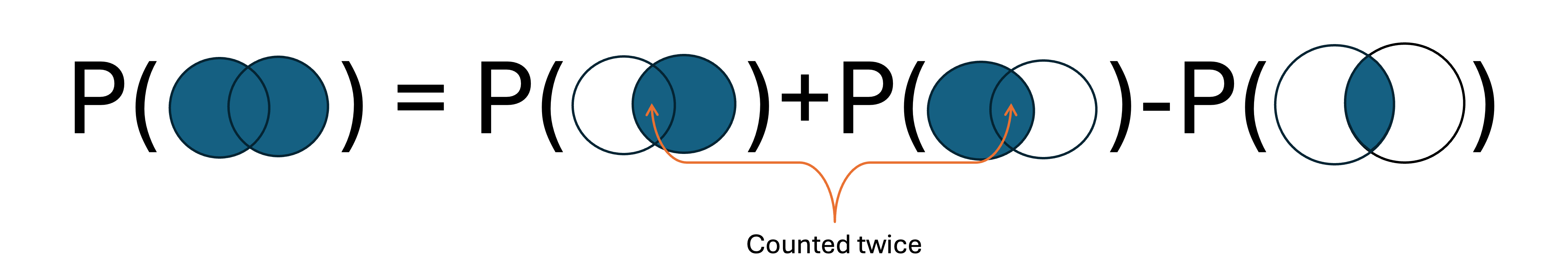
Fig. 4.10 Graphical illustration of the general addition rule
The key component of the general addition rule is the final subtraction of the intersection probability. If we simply add \(P(A)\) and \(P(B)\), we would count the outcomes in the intersection twice. Subtracting \(P(A ∩ B)\) corrects for this double-counting.
i. A Special Case: Mutually Exclusive Events
If \(A\) and \(B\) are mutually exclusive (\(A \cap B = \emptyset\)),
\[P(A \cup B) = P(A) + P(B).\]
This is a restatement of the third axiom of probability, but it can also be seen as a special case of the general addition rule. When the rule is applied to the disjoint events \(A\) and \(B\), the third term disappears because \(P(A \cap B) = P(\emptyset) = 0\).
Avoid the common mistake ‼️
Any special case formulas should only be used when the conditions for the special situation are fully met. When unsure, always begin with the general version.
ii. Extension to Multiple Events
This two-way general addition rule is a special case of the broader inclusion-exclusion principle, which provides a way to decompose the union probability of two or more events. For \(n\) events \(A_1, A_2, ..., A_n\), the inclusion-exclusion principle is constructed following the steps below:
Add the probabilities of individual events.
Subtract the probabilities of all pairwise intersections.
Add the probabilities of all triple intersections.
Subtract the probabilities of all quadruple intersections.
Continue this pattern, with the sign alternating for each step.
Applying the principle to three events \(A\), \(B\), and \(C\), the probability of their union is:
\[\begin{split}P(A \cup B \cup C) &= P(A) + P(B) + P(C) - P(A \cap B) - \\ &P(A \cap C) - P(B \cap C) + P(A \cap B \cap C)\end{split}\]
Example 💡: Two Dice Probability
Continued from the previous examples of throwing two dice.
Compute \(P(A\cup C)\) using the general addition rule, and confirm that the answer is the same as our previous approach without the rule.
\(A\cap C = \{(3,3)\}\). Using the rule and the fact that all outcomes are equally likely,
\[\begin{split}P(A\cup C) &= P(A) + P(C) - P(A\cap C) \\ &= \frac{|A|}{|\Omega|} + \frac{|C|}{|\Omega|} - \frac{|A\cap C|}{|\Omega|} \\ &= \frac{4}{24} + \frac{4}{24} - \frac{1}{24} = \frac{7}{24}.\end{split}\]Compute the probability that the outcome is a double or the sum is equal to 10.
The probability can be written as \(P(B \cup C)\). Since the two events are mutually exclusive, we can use the special addition rule:
\[P(B \cup C) = P(B) + P(C) = \frac{1}{24} + \frac{4}{24} = \frac{5}{24}.\]
4.2.5. Bringing It All Together
Key Takeaways 📝
Probability is a function that maps events to values between 0 and 1, representing the likelihood of those events occurring.
A valid probability function must satisfy three axioms: non-negativity, normalization (sample space has probability 1), and additivity for mutually exclusive events.
The complement rule: \(P(A') = 1 - P(A)\). It is useful for calculating probabilities of events defined by “at least one” or “none.”
The general addition rule: \(P(A \cup B) = P(A) + P(B) - P(A \cap B)\). It can be extended to cases with multiple events using inclusion-exclusion principle.
In the next chapter, we’ll build on these concepts to explore conditional probability and independence, which allow us to analyze how events influence each other.
4.2.6. Exercises
These exercises build your skills in applying probability axioms and rules to calculate probabilities of events.
Exercise 1: Equally Likely Outcomes
A quality control system randomly selects one circuit board from a batch for inspection. The batch contains boards labeled 1 through 20. Define the following events:
\(A\) = “Board number is a multiple of 3”
\(B\) = “Board number is greater than 12”
\(C\) = “Board number is odd”
Assuming each board is equally likely to be selected:
List the elements of \(A\), \(B\), and \(C\).
Calculate \(P(A)\), \(P(B)\), and \(P(C)\).
Find \(A \cap B\) and calculate \(P(A \cap B)\).
Calculate \(P(A \cup B)\) using the general addition rule.
Are events \(A\) and \(C\) mutually exclusive? Justify your answer and calculate \(P(A \cup C)\).
Solution
Part (a): List Elements
\(A = \{3, 6, 9, 12, 15, 18\}\) — multiples of 3 from 1 to 20
\(B = \{13, 14, 15, 16, 17, 18, 19, 20\}\) — numbers greater than 12
\(C = \{1, 3, 5, 7, 9, 11, 13, 15, 17, 19\}\) — odd numbers
Part (b): Individual Probabilities
Since all outcomes are equally likely, \(P(\text{event}) = \frac{|\text{event}|}{|\Omega|}\)
\(P(A) = \frac{6}{20} = 0.30\)
\(P(B) = \frac{8}{20} = 0.40\)
\(P(C) = \frac{10}{20} = 0.50\)
Part (c): Intersection A ∩ B
\(A \cap B = \{15, 18\}\) — boards that are both multiples of 3 AND greater than 12
\(P(A \cap B) = \frac{2}{20} = 0.10\)
Part (d): P(A ∪ B) Using General Addition Rule
Verification: \(A \cup B = \{3, 6, 9, 12, 13, 14, 15, 16, 17, 18, 19, 20\}\) has 12 elements, and \(\frac{12}{20} = 0.60\) ✓
Part (e): Are A and C Mutually Exclusive?
No, A and C are NOT mutually exclusive.
\(A \cap C = \{3, 9, 15\} \neq \emptyset\)
There are odd multiples of 3 (namely 3, 9, and 15), so the events can occur simultaneously.
To calculate \(P(A \cup C)\):
Exercise 2: Complement Rule Applications
A software testing team runs automated tests on a program. Each test can result in one of four outcomes: {Pass, Minor Bug, Major Bug, Crash}. Based on historical data:
\(P(\text{Pass}) = 0.72\)
\(P(\text{Minor Bug}) = 0.15\)
\(P(\text{Major Bug}) = 0.08\)
\(P(\text{Crash}) = 0.05\)
Verify that this is a valid probability distribution.
Calculate the probability that the test does NOT pass.
Let \(F\) = “test finds a defect” (Minor Bug, Major Bug, or Crash). Calculate \(P(F)\) using the complement rule.
Let \(S\) = “test reveals a serious issue” (Major Bug or Crash). Calculate \(P(S')\).
If 100 tests are run independently, approximately how many would you expect to find defects?
Solution
Part (a): Verify Valid Distribution
Check the probability axioms:
Non-negativity: All probabilities ≥ 0 ✓
Normalization: Sum = 0.72 + 0.15 + 0.08 + 0.05 = 1.00 ✓
Yes, this is a valid probability distribution.
Part (b): Probability of NOT Passing
Using the complement rule:
Part (c): P(F) Using Complement Rule
The event \(F\) = “finds a defect” is the complement of “Pass”:
\(F = \{\text{Minor Bug, Major Bug, Crash}\} = \text{Pass}'\)
Alternatively, using additivity (since outcomes are mutually exclusive):
Part (d): P(S’)
\(S = \{\text{Major Bug, Crash}\}\)
Part (e): Expected Defects in 100 Tests
Expected number of tests finding defects = \(100 \times P(F) = 100 \times 0.28 = 28\) tests.
Exercise 3: General Addition Rule
In a computer science department survey of 200 students:
120 students know Python
85 students know Java
50 students know both Python and Java
Let \(P\) = “student knows Python” and \(J\) = “student knows Java.”
Calculate \(P(P)\), \(P(J)\), and \(P(P \cap J)\).
Calculate \(P(P \cup J)\) — the probability a randomly selected student knows at least one of the languages.
Calculate the probability that a student knows Python but NOT Java.
Calculate the probability that a student knows exactly one of the two languages.
Calculate the probability that a student knows neither language.
Solution
Part (a): Basic Probabilities
\(P(P) = \frac{120}{200} = 0.60\)
\(P(J) = \frac{85}{200} = 0.425\)
\(P(P \cap J) = \frac{50}{200} = 0.25\)
Part (b): P(P ∪ J) — At Least One Language
Using the general addition rule:
Part (c): Python but NOT Java
We want \(P(P \cap J')\)
This represents students who know Python only.
Part (d): Exactly One Language
“Exactly one” = (Python only) OR (Java only)
Python only: \(P(P \cap J') = 0.35\)
Java only: \(P(P' \cap J) = P(J) - P(P \cap J) = 0.425 - 0.25 = 0.175\)
Alternatively: \(P(\text{exactly one}) = P(P \cup J) - P(P \cap J) = 0.775 - 0.25 = 0.525\) ✓
Part (e): Neither Language
Using the complement rule:
Exercise 4: Two Dice Problem
Two fair six-sided dice are rolled. Let the outcome be the ordered pair \((d_1, d_2)\) where \(d_1\) is the result of the first die and \(d_2\) is the result of the second die.
How many outcomes are in the sample space \(\Omega\)?
Define the event \(S_7\) = “the sum equals 7.” List the outcomes in \(S_7\) and calculate \(P(S_7)\).
Define the event \(D\) = “both dice show the same value” (doubles). List the outcomes in \(D\) and calculate \(P(D)\).
Are \(S_7\) and \(D\) mutually exclusive? Calculate \(P(S_7 \cup D)\).
Define \(E\) = “at least one die shows an even number.” Calculate \(P(E)\) using the complement rule.
Calculate the probability that the sum is at least 10.
Solution
Part (a): Size of Sample Space
Each die has 6 outcomes, and the dice are distinguishable (ordered pair).
\(|\Omega| = 6 \times 6 = 36\)
Part (b): Sum Equals 7
\(S_7 = \{(1,6), (2,5), (3,4), (4,3), (5,2), (6,1)\}\)
\(|S_7| = 6\)
Part (c): Doubles
\(D = \{(1,1), (2,2), (3,3), (4,4), (5,5), (6,6)\}\)
\(|D| = 6\)
Part (d): Are S₇ and D Mutually Exclusive?
Yes, they are mutually exclusive.
\(S_7 \cap D = \emptyset\) because no double can sum to 7. (Doubles sum to 2, 4, 6, 8, 10, or 12.)
Since they’re mutually exclusive:
Part (e): At Least One Even Die
Use the complement rule. Let \(E'\) = “both dice show odd numbers.”
Odd values: {1, 3, 5} — each die has 3 odd values.
\(|E'| = 3 \times 3 = 9\) (all combinations of two odd values)
Part (f): Sum at Least 10
List outcomes where \(d_1 + d_2 \geq 10\):
Sum = 10: (4,6), (5,5), (6,4) — 3 outcomes
Sum = 11: (5,6), (6,5) — 2 outcomes
Sum = 12: (6,6) — 1 outcome
Total: 6 outcomes
Exercise 5: Inclusion-Exclusion for Three Events
A tech company surveyed 500 employees about which development tools they use:
280 use VS Code (\(V\))
220 use PyCharm (\(P\))
150 use Sublime (\(S\))
100 use both VS Code and PyCharm
70 use both VS Code and Sublime
50 use both PyCharm and Sublime
30 use all three tools
Calculate \(P(V)\), \(P(P)\), \(P(S)\), \(P(V \cap P)\), \(P(V \cap S)\), \(P(P \cap S)\), and \(P(V \cap P \cap S)\).
Using the inclusion-exclusion principle, calculate the probability that a randomly selected employee uses at least one of the three tools.
What is the probability that an employee uses none of these three tools?
What is the probability that an employee uses exactly one of the three tools?
Solution
Part (a): Individual Probabilities
\(P(V) = \frac{280}{500} = 0.56\)
\(P(P) = \frac{220}{500} = 0.44\)
\(P(S) = \frac{150}{500} = 0.30\)
\(P(V \cap P) = \frac{100}{500} = 0.20\)
\(P(V \cap S) = \frac{70}{500} = 0.14\)
\(P(P \cap S) = \frac{50}{500} = 0.10\)
\(P(V \cap P \cap S) = \frac{30}{500} = 0.06\)
Part (b): At Least One Tool (Inclusion-Exclusion)
Part (c): None of the Tools
This means 8% of employees (40 people) don’t use any of these three tools.
Part (d): Exactly One Tool
Use the principle: count each region separately.
V only = V − (those using V with others) = \(P(V) - P(V \cap P) - P(V \cap S) + P(V \cap P \cap S)\) = 0.56 − 0.20 − 0.14 + 0.06 = 0.28
P only = \(P(P) - P(V \cap P) - P(P \cap S) + P(V \cap P \cap S)\) = 0.44 − 0.20 − 0.10 + 0.06 = 0.20
S only = \(P(S) - P(V \cap S) - P(P \cap S) + P(V \cap P \cap S)\) = 0.30 − 0.14 − 0.10 + 0.06 = 0.12
Exercise 6: Verifying Probability Axioms
Determine whether each of the following could be a valid probability assignment. If not, identify which axiom is violated.
\(P(A) = 0.5, P(B) = 0.6, P(A \cap B) = 0.7\)
\(P(A) = 0.3, P(A') = 0.8\)
For sample space \(\Omega = \{1, 2, 3, 4\}\): \(P(\{1\}) = 0.2, P(\{2\}) = 0.3, P(\{3\}) = 0.3, P(\{4\}) = 0.2\)
\(P(A) = 1.2\) for some event \(A\)
For mutually exclusive events A and B: \(P(A) = 0.4, P(B) = 0.5, P(A \cup B) = 0.8\)
\(P(A) = 0.6, P(B) = 0.7, P(A \cup B) = 1.0\)
Solution
Part (a): Invalid
Axiom violated: The intersection cannot have higher probability than either individual event.
Since \(A \cap B \subseteq A\), we must have \(P(A \cap B) \leq P(A)\).
Here, \(P(A \cap B) = 0.7 > P(A) = 0.5\). This violates the monotonicity property derived from the axioms.
Part (b): Invalid
Axiom violated: Normalization (via complement rule).
We must have \(P(A) + P(A') = 1\), but \(0.3 + 0.8 = 1.1 \neq 1\).
Part (c): Valid
Check the axioms:
Non-negativity: All probabilities ≥ 0 ✓
Normalization: 0.2 + 0.3 + 0.3 + 0.2 = 1.0 ✓
Additivity: For simple events (singletons), this is satisfied by construction.
Part (d): Invalid
Axiom violated: Probabilities must be bounded above by 1.
\(P(A) = 1.2 > 1\) violates the normalization axiom (since \(A \subseteq \Omega\) and \(P(\Omega) = 1\)).
Part (e): Invalid
Axiom violated: Additivity for mutually exclusive events.
For mutually exclusive events: \(P(A \cup B) = P(A) + P(B)\)
Here: \(P(A) + P(B) = 0.4 + 0.5 = 0.9 \neq 0.8 = P(A \cup B)\)
Part (f): Valid (possibly)
Check the general addition rule:
Since \(0 \leq P(A \cap B) = 0.3 \leq \min(P(A), P(B)) = 0.6\), this is valid.
The events overlap with \(P(A \cap B) = 0.3\), and their union covers the entire sample space.
4.2.7. Additional Practice Problems
True/False Questions (1 point each)
If \(P(A) = 0.4\) and \(P(B) = 0.5\), then \(P(A \cup B)\) must equal 0.9.
Ⓣ or Ⓕ
The probability of any event is always between 0 and 1, inclusive.
Ⓣ or Ⓕ
If \(A\) and \(B\) are mutually exclusive, then \(P(A \cap B) = P(A) \cdot P(B)\).
Ⓣ or Ⓕ
For any event \(A\), \(P(A) + P(A') = 1\).
Ⓣ or Ⓕ
If \(A \subseteq B\), then \(P(A) \leq P(B)\).
Ⓣ or Ⓕ
The general addition rule \(P(A \cup B) = P(A) + P(B) - P(A \cap B)\) applies only when A and B are mutually exclusive.
Ⓣ or Ⓕ
Multiple Choice Questions (2 points each)
If \(P(A) = 0.35\) and \(P(B) = 0.60\), and A and B are mutually exclusive, what is \(P(A \cup B)\)?
Ⓐ 0.21
Ⓑ 0.95
Ⓒ 0.25
Ⓓ Cannot be determined
A fair six-sided die is rolled. What is the probability of rolling an even number or a number greater than 4?
Ⓐ 1/2
Ⓑ 2/3
Ⓒ 5/6
Ⓓ 1
If \(P(A) = 0.6\), \(P(B) = 0.5\), and \(P(A \cup B) = 0.8\), what is \(P(A \cap B)\)?
Ⓐ 0.1
Ⓑ 0.3
Ⓒ 0.5
Ⓓ 1.1
In a batch of 100 items, 15 are defective. If one item is randomly selected, what is the probability that it is NOT defective?
Ⓐ 0.15
Ⓑ 0.75
Ⓒ 0.85
Ⓓ 0.90
Answers to Practice Problems
True/False Answers:
False — This would only be true if A and B were mutually exclusive. Without knowing \(P(A \cap B)\), we cannot determine \(P(A \cup B)\). The general addition rule requires subtracting \(P(A \cap B)\).
True — By the axioms of probability: \(P(A) \geq 0\) (non-negativity) and \(P(A) \leq P(\Omega) = 1\) (normalization).
False — If A and B are mutually exclusive, \(P(A \cap B) = 0\), not \(P(A) \cdot P(B)\). The formula \(P(A \cap B) = P(A) \cdot P(B)\) applies to independent events, which is a different concept.
True — This is the complement rule, derived from Axioms 2 and 3.
True — If A is a subset of B, every outcome in A is also in B. Therefore, \(P(A) \leq P(B)\).
False — The general addition rule applies to all pairs of events. For mutually exclusive events, it simplifies to \(P(A \cup B) = P(A) + P(B)\) because \(P(A \cap B) = 0\).
Multiple Choice Answers:
Ⓑ — For mutually exclusive events: \(P(A \cup B) = P(A) + P(B) = 0.35 + 0.60 = 0.95\).
Ⓑ — Even numbers: {2, 4, 6}. Numbers > 4: {5, 6}. Union: {2, 4, 5, 6} = 4 outcomes. \(P = \frac{4}{6} = \frac{2}{3}\).
Ⓑ — Using the general addition rule: \(P(A \cap B) = P(A) + P(B) - P(A \cup B) = 0.6 + 0.5 - 0.8 = 0.3\).
Ⓒ — Using the complement rule: \(P(\text{not defective}) = 1 - P(\text{defective}) = 1 - 0.15 = 0.85\).