Slides 📊

Download Chapter 5 slides (PPTX)

5.5. Covariance of Dependent Random Variables

Many real-world scenarios involve random variables that influence each other—driving violations may correlate with accident rates, stock prices often move together, and rainfall affects crop yields. When random variables are dependent, their joint behavior becomes more complex, requiring us to understand how they vary together.

Road Map 🧭

• Introduce covariance, a measure of how random variables change together.

• Define correlation as a standardized measure of relationship strength.

• Extend variance formulas to sums of dependent random variables.

• Explore the independence property and its effect on covariance.

5.5.1. Beyond Independence: Understanding Covariance

When analyzing two random variables \(X\) and \(Y\) together, we often ask: when \(X\) is large, does \(Y\) also tend to be large, or do they usually move in the opposite directions? Covariance provides a mathematical way to measure this relationship.

Definition

The covariance between two discrete random variables \(X\) and \(Y\), denoted \(\text{Cov}(X,Y)\) or \(\sigma_{XY}\), is defined as:

\[\sigma_{XY} = \text{Cov}(X,Y) = E[(X - \mu_X)(Y - \mu_Y)]\]

Interpreting the formula

• If \(X\) and \(Y\) tend to be simultaneously above their means or simultaneously below their means, their covariance will be positive.

• If \(Y\) tends to be below its mean when \(X\) is above its mean, and vice versa, their covariance will be negative.

• If \(X\) and \(Y\) have no systematic relationship, their covariance will be close to zero.

• In general, the covariance describes the strength (magnitude) and direction (sign) of the linear relationship between \(X\) and \(Y\).

Computational shortcut

Covariance has a computational shortcut similar to that of variance.

\[\sigma_{XY}= E[XY] - \mu_X\mu_Y.\]

Its derivation is analogous to the derivation of the shortcut for variance. We leave its step-by-step demonstration as an indepdent exercise.

Also note that computing covariance requires working with the joint probability mass function because:

\[E[XY] = \sum_{(x,y)\in \text{supp}(X,Y)} xy \, p_{X,Y}(x,y)\]

Example💡: Salamander Insurance Company (SIC), Continued

Recall Salamander Insurance Company (SIC), who keeps track of the proababilities of moving violations (\(X\)) and accidents (\(Y\)) made by there customers.

\(x\) \ \(y\)	0	1	2	\(p_X(x)\)
0	0.58	0.015	0.005	0.60
1	0.18	0.058	0.012	0.25
2	0.02	0.078	0.002	0.10
3	0.02	0.029	0.001	0.05
\(p_Y(y)\)	0.80	0.18	0.02	1

SIC wants to know whether the number of moving violations (\(X\)) and the number accidents (\(Y\)) made by a customer are linearly associated. To answer this question, we must compute the covariance of the two random variables.

We already know:

• \(E[X] = 0.6\) (average number of moving violations)

• \(E[Y] = 0.22\) (average number of accidents)

from the previous examples. To calculate the covariance, we need to find \(E[XY]\).

\[\begin{split}E[XY] =& \sum_{(x,y)\in \text{supp}(X,Y)} xy \, p_{X,Y}(x,y) \\ =& 1 \cdot 1 \cdot 0.058 + 1 \cdot 2 \cdot 0.012 + 2 \cdot 1 \cdot 0.078 \\ &+ 2 \cdot 2 \cdot 0.002 + 3 \cdot 1 \cdot 0.029 + 3 \cdot 2 \cdot 0.001 \\ =& 0.339\end{split}\]

Now we can compute the covariance:

\[\begin{split}\text{Cov}(X,Y) &= E[XY] - E[X]E[Y] = 0.339 - 0.6 \cdot 0.22\\ &= 0.339 - 0.132 = 0.207\end{split}\]

The positive covariance indicates that customers with more moving violations tend to have more accidents, which aligns with our intuition about driving behavior. However, it is not easy to assess the strength of this relationship with covariance alone. To evaluate the strength more objectively, we now turn to our next topic.

5.5.2. Correlation: A Standardized Measure

The sign of the covariance tells us the direction of the relationship, but its magnitude is difficult to interpret since it depends on the scales of \(X\) and \(Y\). For instance, if we measured \(X\) in inches and then converted to centimeters, the covariance would change even though the underlying relationship remains the same.

To address the scale dependency of covariance, we use correlation, which standardizes covariance to a value between -1 and +1.

Definition

The correlation between two discrete random variables \(X\) and \(Y\), denoted \(\rho_{XY}\), is defined as:

\[\rho_{XY} = \frac{\sigma_{XY}}{\sigma_X \sigma_Y}.\]

From the formula, we can say that the correlation is obtained by taking the covariance, then removing the scales of \(X\) and \(Y\) by diving by both \(\sigma_X\) and \(\sigma_Y\).

This standardization provides several advantages:

• Correlation is always between -1 and +1.

• A correlation of +1 indicates a perfect positive linear relationship.

• A correlation of -1 indicates a perfect negative linear relationship.

• A correlation of 0 suggests no linear relationship.

• Being unitless, correlation allows for meaningful comparisons across different variable pairs.

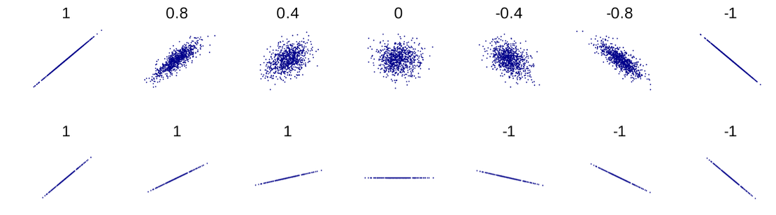
Fig. 5.8 Plots of joint distributions witth varying degrees of correlation

Eaxample💡: Salamander Insurance Company (SIC), Continued

Let us compute the correlation between \(X\) and \(Y\) for an objective assessment of the strength of their linear relationship.

\(x\) \ \(y\)	0	1	2	\(p_X(x)\)
0	0.58	0.015	0.005	0.60
1	0.18	0.058	0.012	0.25
2	0.02	0.078	0.002	0.10
3	0.02	0.029	0.001	0.05
\(p_Y(y)\)	0.80	0.18	0.02	1

We already know:

• \(E[X] = 0.6\) (average number of moving violations)

• \(E[Y] = 0.22\) (average number of accidents)

• \(E[X^2] = 1.1\)

• \(Cov(X,Y) = 0.207\)

from the previous examples. To use the formula for correlation, we must find the standard deviations of \(X\) and \(Y\).

\[\begin{split}Var(X) &= E[X^2] - (E[X])^2\\ &= 1.1 - (0.6)^2 = 0.74\\ \sigma_X & = \sqrt{0.74} \approx 0.8602\end{split}\]

\[\begin{split}Var(Y) &= E[Y^2] - (E[Y])^2 \\ &= [(1^2)(0.18) + (2^2)(0.02)]- (0.22)^2\\ &= 0.26 - 0.0484 = 0.2116\\ \sigma_Y &= \sqrt{0.2116} = 0.46.\end{split}\]

Now the correlation is

\[\rho_{X,Y} = \frac{\text{Cov}(X,Y)}{\sigma_X \sigma_Y} = \frac{0.207}{(0.8602)(0.46)} \approx 0.5231.\]

We now see that the positive linear association between \(X\) and \(Y\) are moderate in strength.

5.5.3. Independence and Covariance

Theorem: Independence implies Zero Covariance

If \(X\) and \(Y\) are independent random variables, then

\[\text{Cov}(X,Y) = 0.\]

Proof of theorem

We use the expectation independence property:

\[\begin{split}\begin{aligned} E[XY] &= \sum_{(x,y)\in \text{supp}(X,Y)} xy \, p_{X,Y}(x,y) \\ &= \sum_{x\in \text{supp}(X)} \sum_{y \in \text{supp}(Y)} xy \, p_X(x)p_Y(y) \\ &= \sum_{x\in \text{supp}(X)} x \, p_X(x) \sum_{y \in \text{supp}(Y)} y \, p_Y(y) \\ &= E[X] \cdot E[Y] = \mu_X \mu_Y \end{aligned}\end{split}\]

The second equality above holds because \(p_{X,Y} (x,y) = p_X(x)p_Y(y)\) for all \((x,y)\) pairs in the support due to independence of \(X\) and \(Y\).

Therefore,

\[\text{Cov}(X,Y) = E[XY] - \mu_X\mu_Y = \mu_X\mu_Y - \mu_X\mu_Y = 0.\]

This property is crucial because it allows us to determine when we can use the simpler variance formulas for sums of independent random variables. If covariance is non-zero, we must account for the dependence.

Zero Covariance Does Not Imply Independence

It’s important to note that the converse of the previous theorem is not always true—a zero covariance does not necessarily imply independence. This is because “no linear relationship” does not rule out other types of relationships. See Fig. 5.9 for some examples:

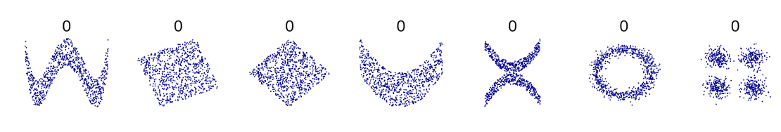
Fig. 5.9 Dependent distributions with zero covariance

5.5.4. Variance of Sums of Dependent Random Variables

When random variables are dependent, the variance of their sum (or difference) includes an additional term that accounts for their covariance:

\[\text{Var}(X \pm Y) = \text{Var}(X) + \text{Var}(Y) \pm 2\text{Cov}(X,Y)\]

For linear combinations:

\[\text{Var}(aX + bY) = a^2\text{Var}(X) + b^2\text{Var}(Y) + 2ab\text{Cov}(X,Y)\]

These formulas highlight a critical insight: dependence between random variables can either increase or decrease the variance of their sum, depending on whether the covariance is positive (variables tend to move together) or negative (variables tend to offset each other).

For n dependent random variables, the formula extends to:

\[\text{Var}(X_1 + X_2 + \ldots + X_n) = \sum_{i=1}^{n} \text{Var}(X_i) + 2 \sum_{i=1}^{n} \sum_{j>i}^{n} \text{Cov}(X_i, X_j)\]

This formula includes the variance of each individual random variable plus the covariance between each pair of variables.

Example💡: SIC, Continued

SIC is planning a promotional offer based on a risk score \(Z = 2X + 5Y\), which combines both factors with different weights. The company wants to know the average value and standard deviation of the sum of these scores for its 35 customers.

\(x\) \ \(y\)	0	1	2	\(p_X(x)\)
0	0.58	0.015	0.005	0.60
1	0.18	0.058	0.012	0.25
2	0.02	0.078	0.002	0.10
3	0.02	0.029	0.001	0.05
\(p_Y(y)\)	0.80	0.18	0.02	1

Calculate the Expected Value of \(Z\)

The expected value of \(Z\) is:

\[\begin{split}E[Z] &= E[2X + 5Y] = 2E[X] + 5E[Y]\\ &= 2 \cdot 0.6 + 5 \cdot 0.22 = 1.2 + 1.1 = 2.3.\end{split}\]

For all 35 customers combined:

\[E[\sum_{i=1}^{35} Z_i] = 35 \cdot E[Z] = 35 \cdot 2.3 = 80.5\]

Calculate the Variance of \(Z\)

For a single customer,

\[\begin{split}\begin{aligned} \text{Var}(Z) &= \text{Var}(2X + 5Y) \\ &= 2^2 \text{Var}(X) + 5^2 \text{Var}(Y) + 2 \cdot 2 \cdot 5 \cdot \text{Cov}(X,Y) \\ &= 4 \cdot 0.74 + 25 \cdot 0.2116 + 20 \cdot 0.207 \\ &= 2.96 + 5.29 + 4.14 \\ &= 12.39 \end{aligned}\end{split}\]

Now, assuming the 35 customers are independent of each other (one customer’s driving behavior doesn’t affect another’s), the variance of the sum is:

\[\text{Var}(\sum_{i=1}^{35} Z_i) = 35 \cdot \text{Var}(Z) = 35 \cdot 12.39 = 433.65\]

Calculate the Standard Deviation

The standard deviation is the square root of the variance:

\[\sigma_{\sum Z_i} = \sqrt{433.65} \approx 20.82\]

This standard deviation tells SIC how much variation is expected in the sum of risk scores across their 35 customers—valuable information for setting appropriate thresholds for their promotional offer.

The Effect of Dependence on Risk Assessment

It’s worth noting how the dependence between moving violations and accidents affects SIC’s risk calculations. If we had incorrectly assumed that X and Y were independent (ignoring their positive covariance of 0.207), the variance calculation would have been:

\[\begin{split}\begin{aligned} \text{Var}_{incorrect}(Z) &= 4 \cdot 0.74 + 25 \cdot 0.2116 \\ &= 2.96 + 5.29 \\ &= 8.25 \end{aligned}\end{split}\]

This would have resulted in an underestimation of the variance by approximately 33% and an underestimation of the standard deviation by about 18%. Such an error could lead to significant mispricing of insurance policies or inadequate risk management.

5.5.5. Bringing It All Together

Key Takeaways 📝

1. Covariance measures how two random variables change together. Positive values indicate that they tend to move in the same direction, and negative values indicate opposite movements.

2. Correlation standardizes covariance to a unitless measure between -1 and +1, making it easier to interpret the strength of relationships regardless of variable scales.

3. Independent random variables have zero covariance, though zero covariance doesn’t necessarily imply independence.

4. The variance of a linear combination of dependent random variables includes an additional term accounting for their covariances: \(\text{Var}(aX + bY) = a^2\text{Var}(X) + b^2\text{Var}(Y) + ab2\text{Cov}(X,Y)\).

5. Positive covariance increases the variance of a sum, while negative covariance decreases it—reflecting how dependencies can either amplify or mitigate variability.

Understanding how random variables covary is essential for modeling complex systems where independence is the exception rather than the rule. While the mathematics becomes more involved when accounting for dependencies, the resulting models more faithfully represent reality, leading to better decisions and predictions.

In our next section, we’ll explore specific named discrete probability distributions that occur frequently in practice, beginning with the binomial distribution—a foundational model for many counting problems.

5.5.6. Exercises

These exercises develop your skills in computing covariance, testing for independence using E[XY] = E[X]E[Y], and calculating variance of sums when random variables are dependent.

Exercise 1: Computing E[XY] from a Joint PMF

A tech company tracks two metrics for their mobile app: \(X\) = number of crashes per day and \(Y\) = user rating (1-3 scale). The joint PMF is:

Table 5.18 Joint PMF for Crashes and Rating

Joint PMF \(p_{X,Y}(x,y)\)
\(x \backslash y\)	1	2	3	\(p_X(x)\)
0	0.05	0.15	0.30	0.50
1	0.10	0.15	0.05	0.30
2	0.10	0.05	0.05	0.20
\(p_Y(y)\)	0.25	0.35	0.40	1.00

1. Calculate \(E[X]\) and \(E[Y]\) using the marginal distributions.

2. Calculate \(E[XY]\) using LOTUS on the joint distribution.

3. Is \(E[XY] = E[X] \cdot E[Y]\)? What does this tell you about X and Y?

4. The company uses a “quality score” defined as \(Q = 10Y - 5X\). Calculate \(E[Q]\).

Solution

Part (a): E[X] and E[Y] from marginals

\[E[X] = (0)(0.50) + (1)(0.30) + (2)(0.20) = 0 + 0.30 + 0.40 = 0.70\]

\[E[Y] = (1)(0.25) + (2)(0.35) + (3)(0.40) = 0.25 + 0.70 + 1.20 = 2.15\]

Part (b): E[XY] using joint distribution

Using LOTUS with \(g(x,y) = xy\):

\[E[XY] = \sum_{x,y} xy \cdot p_{X,Y}(x,y)\]

Only terms where both x > 0 and y > 0 contribute:

\[\begin{split}\begin{aligned} E[XY] &= (1)(1)(0.10) + (1)(2)(0.15) + (1)(3)(0.05) \\ &\quad + (2)(1)(0.10) + (2)(2)(0.05) + (2)(3)(0.05)\\ &= 0.10 + 0.30 + 0.15 + 0.20 + 0.20 + 0.30 = 1.25 \end{aligned}\end{split}\]

Part (c): Testing E[XY] = E[X]·E[Y]

\[E[X] \cdot E[Y] = 0.70 \times 2.15 = 1.505\]

Since \(E[XY] = 1.25 \neq 1.505 = E[X] \cdot E[Y]\), X and Y are not independent.

Furthermore, since \(E[XY] < E[X] \cdot E[Y]\), this indicates a negative covariance: more crashes tend to occur with lower ratings.

Part (d): E[Q] = E[10Y - 5X]

Using linearity and additivity:

\[E[Q] = E[10Y - 5X] = 10E[Y] - 5E[X] = 10(2.15) - 5(0.70) = 21.5 - 3.5 = 18.0\]

---

Exercise 2: Computing Covariance and Correlation

Continuing with the app data from Exercise 1, where \(E[X] = 0.70\), \(E[Y] = 2.15\), and \(E[XY] = 1.25\).

1. Calculate \(\text{Cov}(X, Y)\) using the shortcut formula.

2. Calculate \(\text{Var}(X)\) and \(\text{Var}(Y)\).

3. Calculate the correlation \(\rho_{XY}\).

4. Interpret the correlation in context.

Solution

Part (a): Cov(X, Y)

Using the shortcut \(\text{Cov}(X,Y) = E[XY] - E[X]E[Y]\):

\[\text{Cov}(X,Y) = 1.25 - (0.70)(2.15) = 1.25 - 1.505 = -0.255\]

The negative covariance confirms that crashes and ratings move in opposite directions.

Part (b): Variances

For \(\text{Var}(X)\):

\[E[X^2] = (0)^2(0.50) + (1)^2(0.30) + (2)^2(0.20) = 0 + 0.30 + 0.80 = 1.10\]

\[\text{Var}(X) = E[X^2] - (E[X])^2 = 1.10 - (0.70)^2 = 1.10 - 0.49 = 0.61\]

For \(\text{Var}(Y)\):

\[E[Y^2] = (1)^2(0.25) + (2)^2(0.35) + (3)^2(0.40) = 0.25 + 1.40 + 3.60 = 5.25\]

\[\text{Var}(Y) = E[Y^2] - (E[Y])^2 = 5.25 - (2.15)^2 = 5.25 - 4.6225 = 0.6275\]

Part (c): Correlation

\[\sigma_X = \sqrt{0.61} \approx 0.781, \quad \sigma_Y = \sqrt{0.6275} \approx 0.792\]

\[\rho_{XY} = \frac{\text{Cov}(X,Y)}{\sigma_X \sigma_Y} = \frac{-0.255}{(0.781)(0.792)} = \frac{-0.255}{0.619} \approx -0.41\]

Part (d): Interpretation

The correlation of ρ ≈ -0.41 indicates a moderate negative linear relationship. Apps with more crashes tend to receive lower ratings, but the relationship is not extremely strong.

---

Exercise 3: Variance of Sums with Dependence

A manufacturing plant tracks defects from two processes. Let \(X\) = defects from Process A and \(Y\) = defects from Process B.

Given information:

• \(E[X] = 3\), \(\text{Var}(X) = 4\)

• \(E[Y] = 2\), \(\text{Var}(Y) = 1\)

• \(\text{Cov}(X, Y) = 1.5\) (positive dependence due to shared equipment)

1. Find \(E[X + Y]\), the expected total defects.

2. Find \(\text{Var}(X + Y)\) accounting for dependence.

3. What would \(\text{Var}(X + Y)\) be if X and Y were independent?

4. Find \(\text{Var}(X - Y)\).

Solution

Part (a): E[X + Y]

\[E[X + Y] = E[X] + E[Y] = 3 + 2 = 5 \text{ defects}\]

Part (b): Var(X + Y) with dependence

\[\text{Var}(X + Y) = \text{Var}(X) + \text{Var}(Y) + 2\text{Cov}(X,Y)\]

\[= 4 + 1 + 2(1.5) = 4 + 1 + 3 = 8\]

Part (c): Var(X + Y) if independent

If independent, \(\text{Cov}(X,Y) = 0\):

\[\text{Var}(X + Y) = \text{Var}(X) + \text{Var}(Y) = 4 + 1 = 5\]

Part (d): Var(X - Y)

\[\text{Var}(X - Y) = \text{Var}(X) + \text{Var}(Y) - 2\text{Cov}(X,Y)\]

\[= 4 + 1 - 2(1.5) = 5 - 3 = 2\]

Notice: Positive covariance increases Var(X + Y) but decreases Var(X - Y).

---

Exercise 4: Portfolio Variance

An investment portfolio contains two stocks with daily returns \(X\) and \(Y\) (in %).

Given:

• \(E[X] = 0.5\%\), \(\text{Var}(X) = 4\)

• \(E[Y] = 0.3\%\), \(\text{Var}(Y) = 9\)

• \(\text{Cov}(X, Y) = -2\) (stocks tend to move in opposite directions)

A portfolio invests 60% in stock X and 40% in stock Y: \(R = 0.6X + 0.4Y\)

1. Find \(E[R]\), the expected portfolio return.

2. Find \(\text{Var}(R)\).

3. What would the portfolio variance be if the stocks were independent?

4. Why is negative covariance beneficial for investors?

Solution

Part (a): E[R]

\[E[R] = 0.6E[X] + 0.4E[Y] = 0.6(0.5) + 0.4(0.3) = 0.30 + 0.12 = 0.42\%\]

Part (b): Var(R)

Using \(\text{Var}(aX + bY) = a^2\text{Var}(X) + b^2\text{Var}(Y) + 2ab\text{Cov}(X,Y)\):

\[\begin{split}\text{Var}(R) &= (0.6)^2(4) + (0.4)^2(9) + 2(0.6)(0.4)(-2) \\ &= 0.36(4) + 0.16(9) + 0.48(-2) \\ &= 1.44 + 1.44 - 0.96 = 1.92\end{split}\]

Part (c): Var(R) if independent

If independent, \(\text{Cov}(X,Y) = 0\):

\[\text{Var}(R) = 0.36(4) + 0.16(9) = 1.44 + 1.44 = 2.88\]

Part (d): Why negative covariance helps

Negative covariance reduces portfolio variance (1.92 vs 2.88). When stock X goes up, stock Y tends to go down, and vice versa. This “hedging” effect smooths out returns.

This is the mathematical basis for diversification: combining assets with negative covariance reduces risk without sacrificing expected return.

---

Exercise 5: Testing Independence

A quality engineer proposes two models for the relationship between machine age \(X\) (years) and defect rate \(Y\) (defects per 100 units):

Model A:

\(x \backslash y\)	2	4	6
1	0.20	0.15	0.05
3	0.10	0.25	0.25

Model B:

\(x \backslash y\)	2	4	6
1	0.12	0.16	0.12
3	0.18	0.24	0.18

1. For Model A, find the marginal PMFs and calculate \(E[X]\), \(E[Y]\), and \(E[XY]\).

2. Is \(E[XY] = E[X] \cdot E[Y]\) for Model A? Are X and Y independent?

3. For Model B, verify that \(p_{X,Y}(x,y) = p_X(x) \cdot p_Y(y)\) for all cells.

4. What’s the key difference between the two models?

Solution

Part (a): Model A calculations

Marginals:

• \(p_X(1) = 0.20 + 0.15 + 0.05 = 0.40\)

• \(p_X(3) = 0.10 + 0.25 + 0.25 = 0.60\)

• \(p_Y(2) = 0.20 + 0.10 = 0.30\)

• \(p_Y(4) = 0.15 + 0.25 = 0.40\)

• \(p_Y(6) = 0.05 + 0.25 = 0.30\)

Expected values:

\[E[X] = (1)(0.40) + (3)(0.60) = 0.40 + 1.80 = 2.20\]

\[E[Y] = (2)(0.30) + (4)(0.40) + (6)(0.30) = 0.60 + 1.60 + 1.80 = 4.00\]

\[E[XY] = (1)(2)(0.20) + (1)(4)(0.15) + (1)(6)(0.05) + (3)(2)(0.10) + (3)(4)(0.25) + (3)(6)(0.25)\]

\[= 0.40 + 0.60 + 0.30 + 0.60 + 3.00 + 4.50 = 9.40\]

Part (b): Independence test for Model A

\[E[X] \cdot E[Y] = 2.20 \times 4.00 = 8.80\]

Since \(E[XY] = 9.40 \neq 8.80 = E[X] \cdot E[Y]\), X and Y are NOT independent in Model A.

Part (c): Model B independence check

Model B has same marginals: \(p_X(1) = 0.40\), \(p_X(3) = 0.60\), \(p_Y(2) = 0.30\), \(p_Y(4) = 0.40\), \(p_Y(6) = 0.30\).

Check products:

• \(p_X(1) \cdot p_Y(2) = 0.40 \times 0.30 = 0.12 = p_{X,Y}(1,2)\) ✓

• \(p_X(1) \cdot p_Y(4) = 0.40 \times 0.40 = 0.16 = p_{X,Y}(1,4)\) ✓

• \(p_X(3) \cdot p_Y(6) = 0.60 \times 0.30 = 0.18 = p_{X,Y}(3,6)\) ✓

All cells satisfy the product rule, so X and Y ARE independent in Model B.

Part (d): Key difference

Both models have identical marginal distributions, but:

• Model A: X and Y are dependent (older machines have higher defect rates)

• Model B: X and Y are independent (age doesn’t affect defect rate)

This shows that marginals alone don’t determine the joint distribution!

---

5.5.7. Additional Practice Problems

True/False Questions (1 point each)

1. If \(\text{Cov}(X, Y) = 0\), then X and Y must be independent.

   Ⓣ or Ⓕ

2. If X and Y are independent, then \(E[XY] = E[X] \cdot E[Y]\).

   Ⓣ or Ⓕ

3. Correlation is always between -1 and +1.

   Ⓣ or Ⓕ

4. \(\text{Var}(X - Y) = \text{Var}(X) - \text{Var}(Y)\) for dependent random variables.

   Ⓣ or Ⓕ

5. Positive covariance means that when X increases, Y always increases.

   Ⓣ or Ⓕ

6. \(\text{Cov}(X, X) = \text{Var}(X)\).

   Ⓣ or Ⓕ

Multiple Choice Questions (2 points each)

7. If \(E[X] = 3\), \(E[Y] = 2\), and \(E[XY] = 8\), what is \(\text{Cov}(X, Y)\)?

   Ⓐ 2

   Ⓑ 6

   Ⓒ 8

   Ⓓ 14

8. Random variables X and Y have \(\text{Var}(X) = 5\), \(\text{Var}(Y) = 8\), and \(\text{Cov}(X, Y) = 3\). What is \(\text{Var}(X + Y)\)?

   Ⓐ 13

   Ⓑ 16

   Ⓒ 19

   Ⓓ 22

9. If \(\text{Cov}(X, Y) = 6\), \(\sigma_X = 2\), and \(\sigma_Y = 4\), what is \(\rho_{XY}\)?

   Ⓐ 0.50

   Ⓑ 0.75

   Ⓒ 1.50

   Ⓓ 3.00

10. Adding a constant to a random variable:

    Ⓐ Changes its variance

    Ⓑ Changes its covariance with other variables

    Ⓒ Changes its expected value but not its variance

    Ⓓ Changes both its expected value and variance

Answers to Practice Problems

True/False Answers:

1. False — Zero covariance means no linear relationship, but X and Y could still be dependent through a non-linear relationship.

2. True — Independence implies \(E[XY] = E[X] \cdot E[Y]\). This is the key property we use to test for independence.

3. True — Correlation \(\rho_{XY} = \frac{\text{Cov}(X,Y)}{\sigma_X \sigma_Y}\) is always in [-1, +1].

4. False — \(\text{Var}(X - Y) = \text{Var}(X) + \text{Var}(Y) - 2\text{Cov}(X,Y)\). Variances add (with covariance adjustment), they don’t subtract.

5. False — Positive covariance means X and Y tend to move together on average, not that they always do.

6. True — \(\text{Cov}(X, X) = E[X^2] - (E[X])^2 = \text{Var}(X)\).

Multiple Choice Answers:

7. Ⓐ — \(\text{Cov}(X,Y) = E[XY] - E[X]E[Y] = 8 - (3)(2) = 8 - 6 = 2\).

8. Ⓒ — \(\text{Var}(X+Y) = \text{Var}(X) + \text{Var}(Y) + 2\text{Cov}(X,Y) = 5 + 8 + 2(3) = 19\).

9. Ⓑ — \(\rho_{XY} = \frac{\text{Cov}(X,Y)}{\sigma_X \sigma_Y} = \frac{6}{(2)(4)} = \frac{6}{8} = 0.75\).

10. Ⓒ — Adding a constant shifts the distribution (changes E[X]) but doesn’t affect spread (Var(X) unchanged) or covariance.