Final Exam — Fall 2025: Worked Solutions

Exam Information

Course: STAT 350 — Introduction to Statistics

Semester: Fall 2025

Total Points: 150 + 15 (Extra Credit) = 165

Time Allowed: 60 minutes

Coverage: Cumulative (Chapters 1–13); primary emphasis on Chapters 12–13, with Chapters 1–7 weighted more heavily than Chapters 8–11 among the earlier material

Problem	Total Possible	Topic
Problem 1 (True/False, 2 pts each)	20	Poisson Independence, Conditional Probability, Card Sampling, E[X·Y] for Dependent RVs, Variance of Linear Combinations, ANOVA Pairs, Tukey HSD Timing, Normal Test Statistic, Residual Patterns, R² Interpretation
Problem 2 (Multiple Choice, 3 pts each)	18	Conditional Probability from Bar Charts, PMF Normalization, CI Duality, Regression Diagnostics, F-statistic Range, ANOVA F Interpretation
Problem 3	18	Venn Diagrams, Intersection and Union of Events
Problem 4	31	Uniform Distribution, Custom PDF (Haoyu), Expected Value, Counterclockwise Symmetry
Problem 5	40	One-Way ANOVA, Pooled SD, Combined SD, Tukey HSD
Problem 6	38	Simple Linear Regression
Total	150 (+ 15 Extra Credit)

—

Problem 1 — True/False (20 points, 2 pts each)

Question 1.1 (2 pts)

Let \(X\) be a Poisson random variable with \(E[X] = \mu\) (average per-hour rate). Suppose we define two Poisson random variables, \(Y\) and \(Z\), defined on two three-hour periods, sharing the rate of \(X\). Then \(Y\) and \(Z\) must be independent and identically distributed, \(\text{Poisson}(3\mu)\).

Solution

Answer: FALSE

Conditionally on \(X = \lambda\), both \(Y \mid X = \lambda\) and \(Z \mid X = \lambda\) are \(\text{Poisson}(3\lambda)\) and independent. However, they share the same random rate \(X\), which induces a positive marginal correlation. By the law of total covariance (and conditional independence of \(Y\) and \(Z\) given \(X\)):

\[\text{Cov}(Y, Z) = \underbrace{E[\text{Cov}(Y,Z \mid X)]}_{=\,0} + \text{Cov}(E[Y \mid X],\, E[Z \mid X]) = \text{Cov}(3X,\, 3X) = 9\,\text{Var}(X) = 9\mu > 0\]

Because \(\text{Cov}(Y, Z) > 0\), \(Y\) and \(Z\) are not marginally independent. The i.i.d. claim fails — the statement is FALSE.

Question 1.2 (2 pts)

Let \(A_1, A_2, \ldots, A_n\) and \(B\) be events from a sample space \(\Omega\) where \(A_1, A_2, \ldots, A_n\) form a partition of \(\Omega\) and \(P(B) > 0\). Then it must follow that \(\sum_{i=1}^{n} P(A_i \mid B) = 1\).

Solution

Answer: TRUE

Since the \(A_i\) partition \(\Omega\), the events \(A_1 \cap B, A_2 \cap B, \ldots, A_n \cap B\) partition \(B\). Therefore:

\[\sum_{i=1}^{n} P(A_i \mid B) = \sum_{i=1}^{n} \frac{P(A_i \cap B)}{P(B)} = \frac{P(B)}{P(B)} = 1\]

Question 1.3 (2 pts)

A special deck of cards contains eight cards: for each number 1, 2, 3, and 4 there is exactly one red card and one black card (so the cards are 1R, 1B, 2R, 2B, 3R, 3B, 4R, 4B). Two cards are drawn at random without replacement, in order. Let \(C\) denote the event that the first card drawn is red, and let \(D\) denote the event that the second card drawn is either a 1 or a 2. Events \(C\) and \(D\) are independent.

Solution

Answer: TRUE

\(P(C) = 4/8 = 1/2\). To find \(P(D \mid C)\), condition on each red first card:

• First is 1R: remaining cards with number 1 or 2: {1B, 2R, 2B} — 3 of 7.

• First is 2R: remaining with number 1 or 2: {1R, 1B, 2B} — 3 of 7.

• First is 3R or 4R: remaining with number 1 or 2: {1R, 1B, 2R, 2B} — 4 of 7.

\[P(D \mid C) = \frac{1}{4}\cdot\frac{3}{7} + \frac{1}{4}\cdot\frac{3}{7} + \frac{1}{4}\cdot\frac{4}{7} + \frac{1}{4}\cdot\frac{4}{7} = \frac{14}{28} = \frac{1}{2}\]

By symmetry, \(P(D \mid C') = 1/2\) as well (verified by the same case analysis for black first cards). Therefore \(P(D) = 1/2 = P(D \mid C)\), confirming that \(C\) and \(D\) are independent.

Question 1.4 (2 pts)

On each day, a factory may be in a high-stress state (\(Y = 1\), probability \(1/4\)) or normal operating mode (\(Y = 0\), probability \(3/4\)). Let \(X\) be the number of machine breakdowns, where \(X \mid Y = 1 \sim \text{Poisson}(10)\) and \(X \mid Y = 0 \sim \text{Poisson}(6)\). Define \(V = X \cdot (1 - Y)\). Since \(V = X \cdot (1 - Y)\), it follows that \(E[V] = E[X] \cdot (1 - E[Y]) = 21/4\).

Solution

Answer: FALSE

The factoring \(E[X \cdot (1-Y)] = E[X] \cdot E[1-Y]\) would be valid only if :math:`X` and :math:`Y` were independent. They are not — \(X\) and \(Y\) are dependent by construction (\(X\)’s distribution changes with \(Y\)).

The correct calculation conditions on \(Y\):

\[E[V] = E[X \cdot (1 - Y)] = E[X(1-Y) \mid Y = 1] \cdot P(Y=1) + E[X(1-Y) \mid Y = 0] \cdot P(Y=0)\]

\[= E[X \cdot 0 \mid Y = 1] \cdot \tfrac{1}{4} + E[X \cdot 1 \mid Y = 0] \cdot \tfrac{3}{4} = 0 + 6 \cdot \tfrac{3}{4} = \tfrac{18}{4} = 4.5\]

The claim that \(E[V] = E[X](1 - E[Y]) = 7 \cdot (3/4) = 21/4 = 5.25\) is incorrect.

Question 1.5 (2 pts)

\(X \sim N(\mu_X = 120, \sigma_X = 15)\) and \(Y \sim N(\mu_Y = 160, \sigma_Y = 20)\) are independent. The planning index is \(I = 0.3X + 0.7Y + 50\). The variance of \(I\) satisfies \(\text{Var}(I) = 0.3 \cdot \text{Var}(X) + 0.7 \cdot \text{Var}(Y) = 347.5\).

Solution

Answer: FALSE

For a linear combination of independent random variables, the variance rule requires squaring the coefficients:

\[\text{Var}(I) = (0.3)^2 \text{Var}(X) + (0.7)^2 \text{Var}(Y) = 0.09 \times 225 + 0.49 \times 400 = 20.25 + 196 = 216.25\]

The statement uses \(0.3 \cdot \text{Var}(X) + 0.7 \cdot \text{Var}(Y) = 0.3(225) + 0.7(400) = 67.5 + 280 = 347.5\), which omits the squaring of the coefficients.

Question 1.6 (2 pts)

In a one-way ANOVA, a Tukey HSD output reports results for 105 unique pairwise comparisons among the group means. The single factor variable in the ANOVA model must have exactly 15 levels.

Solution

Answer: TRUE

The number of unique pairwise comparisons among \(k\) groups is \(\binom{k}{2} = k(k-1)/2\). Setting this equal to 105:

\[\frac{k(k-1)}{2} = 105 \implies k^2 - k - 210 = 0 \implies k = \frac{1 + \sqrt{841}}{2} = \frac{1 + 29}{2} = 15\]

The factor must have exactly 15 levels.

Question 1.7 (2 pts)

A one-way ANOVA is conducted, all assumptions are found reasonable, the F-test statistic is approximately 1 with a large p-value, and the null hypothesis of equal treatment means is not rejected. In this situation, the appropriate next step is to carry out a Tukey multiple comparison procedure to determine which specific treatment means differ.

Solution

Answer: FALSE

The Tukey HSD post-hoc procedure is carried out only after rejecting the ANOVA null hypothesis, to identify which specific pairs of means differ. When \(H_0\) is not rejected (F ≈ 1, large p-value), there is no evidence that any means differ, and performing Tukey HSD would be both statistically inappropriate and uninterpretable. The appropriate conclusion is simply to fail to reject \(H_0\) and report no evidence of differences among treatment means.

Question 1.8 (2 pts)

In simple linear regression \(y_i = \beta_0 + \beta_1 x_i + \varepsilon_i\) where the \(\varepsilon_i\) are i.i.d. normal with variance \(\sigma^2\). Under \(H_0\colon \beta_1 = 0\), if \(\sigma^2\) is known, the test statistic \(\hat{\beta}_1 \div \sqrt{\sigma^2 / S_{XX}}\) follows a standard normal distribution.

Solution

Answer: TRUE

Since the \(\varepsilon_i\) are i.i.d. \(N(0, \sigma^2)\), the least-squares estimator satisfies \(\hat{\beta}_1 \sim N(\beta_1,\, \sigma^2 / S_{XX})\). Under \(H_0\colon \beta_1 = 0\):

\[\frac{\hat{\beta}_1}{\sqrt{\sigma^2 / S_{XX}}} \sim N(0, 1)\]

When \(\sigma^2\) is unknown and replaced by \(s^2 = \text{MSE}\), the statistic follows a \(t\)-distribution with \(n - 2\) degrees of freedom. With \(\sigma^2\) known, the standard normal applies.

Question 1.9 (2 pts)

In a simple linear regression setting, a residual plot shows points randomly scattered around the horizontal line at 0 with roughly the same vertical spread for all values of \(x\), and no clear curvature or funnel shape. This residual pattern provides reasonable support for both the linearity assumption and the constant variance (homoscedasticity) assumption.

Solution

Answer: TRUE

A residual plot where points are (1) randomly scattered around zero with no curvature and (2) maintain roughly constant vertical spread across all \(x\)-values is precisely what we expect when both the linearity assumption and the homoscedasticity assumption hold. Curvature in the residual plot would indicate a violation of linearity; a fan or funnel shape would indicate heteroscedasticity. Neither is present, so both assumptions receive support.

Question 1.10 (2 pts)

In a simple linear regression analysis, the sample coefficient of determination \(R^2\) is found to be very close to 1. From this, we can conclude that a large proportion of the variability in the response variable is explained by its linear relationship with the explanatory variable, and that the relationship between them is in fact linear.

Solution

Answer: FALSE

\(R^2 \approx 1\) does confirm that the fitted linear model explains a large proportion of the variability in \(Y\). However, it does not prove that the true underlying relationship is linear. A nonlinear relationship can still yield a high \(R^2\) over a restricted range of \(x\) values, and the linear model could be a good approximation without being the true mechanism. Assessing linearity requires examining diagnostic plots (scatter plot, residual plot), not just \(R^2\).

—

Problem 2 — Multiple Choice (18 points, 3 pts each)

Question 2.1 (3 pts)

Three elevators in the Math building malfunction during the day (8 am–7 pm) but tend to work normally at night (7 pm–8 am). Let \(X \in \{\text{day}, \text{night}\}\) and \(Y\) = number of working elevators. The conditional distributions of \(Y\) given \(X\) are displayed in the bar graphs below.

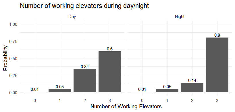
Which of the following probabilities is computed correctly?

• 1. \(P(Y \leq 1) = 0.12\)

• 2. \(P(\{X = \text{day}\} \cap \{Y = 3\}) = 0.6\)

• 3. \(P(X = \text{day}) = P(X = \text{night}) = 1\)

• 4. \(P(Y > 1 \mid X = \text{night}) = 0.94\)

• 5. All of the above

Solution

Answer: (D)

Reading directly from the Night bar chart:

\[P(Y > 1 \mid X = \text{night}) = P(Y = 2 \mid X = \text{night}) + P(Y = 3 \mid X = \text{night}) = 0.14 + 0.80 = 0.94 \checkmark\]

• (A) FALSE. \(P(Y \leq 1)\) is a marginal probability. The bar charts show only the conditional distributions \(P(Y \mid X)\), and \(P(X = \text{day})\) and \(P(X = \text{night})\) are not given, so this marginal cannot be computed from the chart alone.

• (B) FALSE. \(P(\{X = \text{day}\} \cap \{Y = 3\}) = P(Y = 3 \mid X = \text{day}) \cdot P(X = \text{day}) = 0.6 \cdot P(X = \text{day})\). Since \(P(X = \text{day})\) is unknown, this joint probability cannot be determined.

• (C) FALSE. \(P(X = \text{day})\) and \(P(X = \text{night})\) are probabilities of a single categorical variable; they must sum to 1, so each must be strictly between 0 and 1.

Question 2.2 (3 pts)

Let \(X\) be a discrete random variable with support \(\{0, 1, 2, 3\}\). Find the constant \(k\) that makes the following a valid pmf:

\[\begin{split}f_X(x) = \begin{cases} 0.45, & x = 0 \\ k/x, & x = 1, 2, 3 \\ 0, & \text{otherwise} \end{cases}\end{split}\]

• 1. \(k = 0.45\)

• 2. \(k = 0.30\)

• 3. \(k = 0.5455\)

• 4. \(k = 0.9124\)

• 5. \(k = 0.5006\)

• 6. \(k = \infty\)

Solution

Answer: (B)

For a valid pmf, probabilities must sum to 1:

\[0.45 + \frac{k}{1} + \frac{k}{2} + \frac{k}{3} = 1\]

\[k\!\left(1 + \frac{1}{2} + \frac{1}{3}\right) = 0.55 \implies k \cdot \frac{11}{6} = 0.55 \implies k = 0.55 \times \frac{6}{11} = \frac{3.3}{11} = \boxed{0.30}\]

Question 2.3 (3 pts)

A simple linear regression is fit to relate product price (\(x\)) to weekly sales (\(Y\)). All standard assumptions are satisfied. A 95% confidence interval for \(\beta_1\) is \((-12.4,\,-4.1)\). At \(\alpha = 0.05\), what is the correct conclusion about the population linear association?

• 1. There is no evidence of a linear association because 0 is not in the interval.

• 2. There is evidence of a linear association because 0 is not in the interval.

• 3. There is evidence that changing price will cause weekly sales to decrease, because 0 is not in the interval.

• 4. We can only conclude that there is a linear association in this particular sample; a CI cannot draw conclusions about the population.

• 5. We cannot draw any conclusion about linear association without also knowing the p-value.

Solution

Answer: (B)

By the duality between confidence intervals and hypothesis tests, a 95% CI for \(\beta_1\) that excludes 0 is equivalent to rejecting \(H_0\colon \beta_1 = 0\) at \(\alpha = 0.05\). Since \((-12.4, -4.1)\) does not contain 0, we have statistically significant evidence of a linear association between price and sales in the population.

• (A) FALSE. The fact that 0 is not in the interval is precisely why we do have evidence of association — not the reverse.

• (C) FALSE. The existence of a linear association does not establish causation. A regression model alone cannot prove that changing price causes a change in sales.

• (D) FALSE. Confidence intervals do generalize to population-level conclusions — that is their purpose.

• (E) FALSE. The CI and the two-sided t-test for \(\beta_1\) are exactly dual; the CI provides the same information as the p-value for this purpose.

Question 2.4 (3 pts)

A researcher fits a simple linear regression model. Which plot is most appropriate for checking the normality assumption of the errors?

• 1. Scatterplot of \(y\) versus \(x\).

• 2. Plot of residuals versus \(x\) values.

• 3. Normal probability plot (QQ-plot) of the residuals.

• 4. Normal probability plot (QQ-plot) of the response.

• 5. Histogram of the response.

• 6. Histogram of the explanatory variable.

Solution

Answer: (C)

The normality assumption in SLR states that the error terms \(\varepsilon_i\) are normally distributed. Since errors are unobservable, we assess this using the residuals as estimates. A normal QQ-plot of the residuals is the standard diagnostic: if the residuals are approximately normal, the points will fall close to the 45° reference line.

• (A), (B) assess linearity and homoscedasticity, not normality.

• (D), (E) plot the raw response \(Y\), whose distribution depends on both \(x\) and the error; it is not the same as the distribution of the errors.

• (F) is irrelevant to normality of errors.

Question 2.5 (3 pts)

The ANOVA F-statistic always falls within which range?

• 1. The positive real numbers \((0, \infty)\).

• 2. The real numbers \((-\infty, \infty)\).

• 3. The negative real numbers \((-\infty, 0)\).

• 4. The real numbers between 0 and 1.

• 5. None of the above.

Solution

Answer: (A)

The F-statistic is \(F_{\text{TS}} = \text{MSA}/\text{MSE}\). Both MSA and MSE are ratios of non-negative sums of squares to positive degrees of freedom, so each is non-negative. The F-statistic is therefore non-negative. In practice, \(F_{\text{TS}} > 0\) whenever there is any variability between groups, which is virtually always the case with real data. The key accepts (A) as the correct answer.

Note

Technically, \(F_{\text{TS}} = 0\) is possible if all group means are identical (SSA = 0). Strictly speaking the range is \([0, \infty)\), but (A) is the best available answer since none of the other options are correct.

Question 2.6 (3 pts)

A researcher compares four insomnia drugs using one-way ANOVA by randomly assigning seniors to one of the four treatments. Which statements correctly describe the relationship between between-drug variation, within-drug variation, and the F-statistic?

• 1. The ANOVA F-statistic is the ratio of between-group variation to within-group variation.

• 2. A large F occurs when differences among the four drug sample means are large relative to the typical person-to-person variability within each drug group.

• 3. The within-drug variation sets the noise level for judging whether observed differences among drug sample means look unusually large.

• 4. An F-statistic near 1 indicates that between-drug variation is about the same size as within-drug variation, so the drug means do not stand out beyond background variability.

• 5. All of the above.

• 6. None of the above.

Solution

Answer: (E)

All four statements accurately describe how the F-statistic works in one-way ANOVA. Each is a correct and complementary description: (A) gives the mathematical definition; (B) describes when F is large; (C) explains the role of MSE as a baseline; and (D) explains the null-hypothesis-consistent case of F ≈ 1.

—

Problem 3 Setup

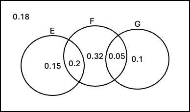
Events \(E\), \(F\), and \(G\) belong to the same sample space \(S\), each with a non-zero probability.

The Venn diagram below shows the probability of each region:

Part (a) uses four Venn diagrams labeled A–D, shown on the exam. The shaded regions correspond to the probability expressions in the matching table.

Problem 3 — Venn Diagrams and Set Theory (18 points)

Question 3a (8 pts)

Match each Venn diagram (A, B, C, or D) with the probability statement that correctly represents its colored region.

Venn Diagram Matching

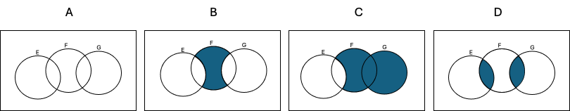
Row	Notation	Venn Diagram Letter
i	\(P(E' \cap F \cap G')\)	B
ii	\(P(E \cap G)\)	A
iii	\(P\!\bigl(F \cap \bigl((E \cap F) \cup G\bigr)\bigr)\)	D
iv	\(P\!\bigl(E' \cap (F \cup G)\bigr)\)	C

Solution

Row i — B: \(E' \cap F \cap G'\) is the part of \(F\) that lies outside both \(E\) and \(G\). In a three-circle diagram this is the region of \(F\) that does not overlap with \(E\) or \(G\) — the center-left “F-only” region. Diagram B shows exactly this.

Row ii — A: \(E \cap G\) is the overlap of \(E\) and \(G\), which includes both the \(E \cap G \cap F'\) region and the \(E \cap G \cap F\) region (\(E \cap F \cap G\)). Diagram A shades all overlapping area between \(E\) and \(G\).

Row iii — D: \(F \cap \bigl((E \cap F) \cup G\bigr) = (E \cap F) \cup (F \cap G)\) — this is the region of \(F\) that overlaps with \(E\) or \(G\) (or both). Diagram D shades the two overlap zones within \(F\).

Row iv — C: \(E' \cap (F \cup G)\) is the part of \(F \cup G\) that falls outside \(E\). This excludes \(E\) but includes everything in \(F\) or \(G\) that \(E\) doesn’t cover. Diagram C shows this region shaded.

Question 3b (10 pts)

Using the Venn diagram probabilities, define events \(A\), \(B\), \(C\), and \(D\) as the colored regions from parts i–iv respectively.

1. (4 pts) Compute \(P(A \cap B \cap C \cap D)\).

2. (6 pts) Compute \(P(A \cup B \cup C \cup D)\).

Solution

(i) From the part (a) matching:

• \(A = E \cap G\). From the Venn diagram probabilities, the region \(E \cap G \cap F'\) (E and G without F) has probability 0; so effectively \(A = E \cap F \cap G\) with \(P(A) = 0.32\).

• \(B = E' \cap F \cap G'\) (F-only region). The diagram shows this region also has probability 0, so \(P(B) = 0\).

Since \(A \subseteq E\) and \(B \subseteq E'\), we have \(A \cap B \subseteq E \cap E' = \emptyset\). Therefore:

\[P(A \cap B \cap C \cap D) \leq P(A \cap B) = 0 \implies \boxed{P(A \cap B \cap C \cap D) = 0}\]

(ii) Identifying \(A \cup B \cup C \cup D\):

• \(A = E \cap G\) (regions within both \(E\) and \(G\))

• \(B = E' \cap F \cap G'\) (F-only)

• \(C = E' \cap (F \cup G)\) (part of \(F \cup G\) outside \(E\))

• \(D = (E \cap F) \cup (F \cap G)\) (overlaps within \(F\))

Together, \(A \cup B \cup C \cup D = F \cup G\) — they cover every region touching \(F\) or \(G\).

Reading probabilities from the Venn diagram for regions in \(F \cup G\):

\[P(A \cup B \cup C \cup D) = P(F \cup G) = 0.20 + 0.32 + 0.05 + 0.10 = \boxed{0.67}\]

(The region \(E' \cap F \cap G'\) = F-only contributes 0 per the diagram, and \(E\)-only (0.15) and outside (0.18) are outside \(F \cup G\).)

—

Problem 4 Setup

Dr. Reese asked two TAs, Zhenghao and Haoyu, to walk clockwise around a rectangular path (length 30 m, width 20 m, total perimeter 100 m), each starting and ending at Dr. Reese’s position. An observation time is chosen uniformly at random from each TA’s lap.

• \(Z\) = distance Zhenghao has traveled from Dr. Reese at the observation time.

• \(H\) = distance Haoyu has traveled from Dr. Reese at the observation time.

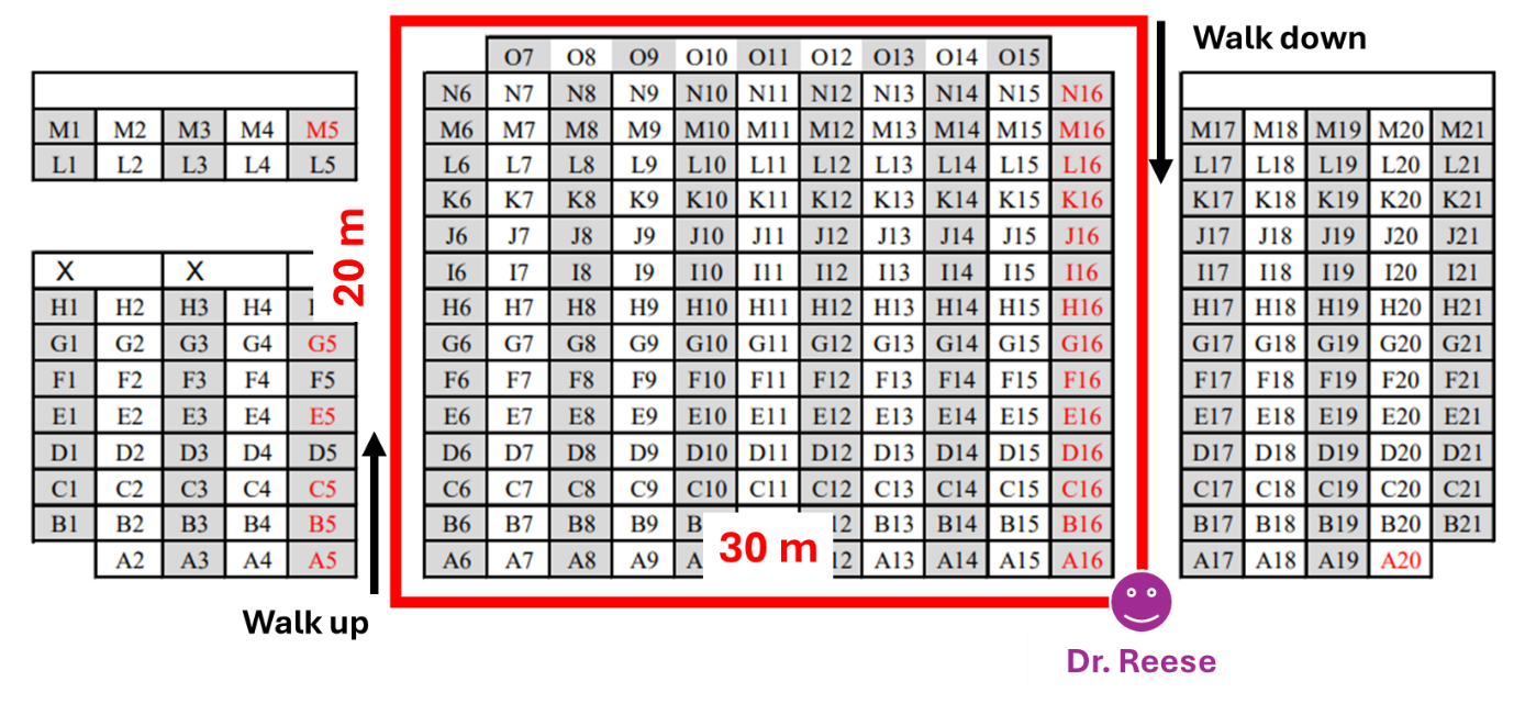
Speed profile for Haoyu (going clockwise from Dr. Reese):

Path Segments

Segment	Distance (m)	Direction	Relative speed
Bottom (horizontal)	[0, 30]	Flat	Baseline
Left side	[30, 50]	Walk up	Half speed (twice as slow)
Top (horizontal)	[50, 80]	Flat	Baseline
Right side	[80, 100]	Walk down	Double speed (twice as fast)

Problem 4 — Uniform and Custom Distributions (31 points)

Question 4a (4 pts)

Determine the distribution of \(Z\) and its parameter(s).

Solution

Zhenghao walks at a constant pace around the 100 m path, and the observation time is chosen uniformly over the entire lap. A uniform observation time on a constant-speed path produces a uniform position on the path:

\[Z \sim \text{Uniform}(a = 0,\; b = 100)\]

Question 4b (4 pts)

What is the probability that Zhenghao is walking up the path at the observation time?

Solution

“Walking up” corresponds to the left-side segment, which spans distances 30 m to 50 m along the path.

\[P(30 < Z < 50) = \frac{50 - 30}{100 - 0} = \frac{20}{100} = \boxed{0.2}\]

Question 4c (10 pts)

Based on Haoyu’s speed, the pdf of \(H\) is:

\[\begin{split}f_H(x) = \begin{cases} k, & 0 < x \leq 30 \\ 2k, & 30 < x \leq 50 \\ k, & 50 < x \leq 80 \\ k/2, & 80 < x \leq 100 \\ 0, & \text{otherwise} \end{cases}\end{split}\]

Determine the value of \(k\) that makes \(f_H(x)\) a valid pdf.

Solution

The pdf must integrate to 1. Since each piece is constant, each integral equals (interval length) × (density):

\[30k + 20(2k) + 30k + 20\!\left(\frac{k}{2}\right) = 1\]

\[30k + 40k + 30k + 10k = 110k = 1\]

\[k = \frac{1}{110} \approx \boxed{0.0091}\]

Intuition: The density is highest on [30, 50] (the up-slope) because Haoyu moves slowly there — a uniformly chosen observation time is more likely to catch him in segments where he spends more time.

Question 4d (6 pts)

What is the probability that Haoyu has traveled between 40 m and 70 m from Dr. Reese?

Solution

The interval [40, 70] spans two pieces of the pdf:

\[P(40 < H < 70) = \int_{40}^{50} 2k\,dx + \int_{50}^{70} k\,dx = 2k(10) + k(20) = \frac{20}{110} + \frac{20}{110} = \frac{40}{110} = \boxed{0.3636}\]

Question 4e (4 pts)

Compare the average travel distance of Zhenghao and Haoyu. Who travels farther on average?

Solution

Zhenghao: \(Z \sim \text{Uniform}(0, 100)\), so \(E[Z] = (0 + 100)/2 = 50\) m.

Haoyu:

\[E[H] = \int_0^{100} x\,f_H(x)\,dx = k\int_0^{30} x\,dx + 2k\int_{30}^{50} x\,dx + k\int_{50}^{80} x\,dx + \frac{k}{2}\int_{80}^{100} x\,dx\]

\[= \frac{1}{110}\cdot\frac{30^2}{2} + \frac{2}{110}\cdot\frac{50^2 - 30^2}{2} + \frac{1}{110}\cdot\frac{80^2-50^2}{2} + \frac{1}{220}\cdot\frac{100^2-80^2}{2}\]

Using the weighted-midpoint shortcut (weight = probability in each segment):

\[E[H] = 15 \cdot \frac{30}{110} + 40 \cdot \frac{40}{110} + 65 \cdot \frac{30}{110} + 90 \cdot \frac{10}{110} = \frac{450 + 1600 + 1950 + 900}{110} = \frac{4900}{110} = \boxed{44.5455}\ \text{m}\]

Since \(E[Z] = 50 > 44.5455 = E[H]\), Zhenghao travels farther on average.

Intuition: The observation time is uniform, but Haoyu moves slowly on the uphill segment [30, 50], so more observation times catch him there (closer to the start). This pulls his average observed position below 50 m.

Note on solution key ⚠️

The solution key’s “Easier Calculation” section states \(E[H] = 4900/110 = 45.5455\). This is a transcription error — \(4900/110 = 44.5455\), not 45.5455. Both the exact integral and the midpoint method confirm \(E[H] = 44.5455\).

Question 4f (3 pts)

Suppose Zhenghao and Haoyu now walk counterclockwise instead of clockwise. Which of the following quantities will change?

• 1. The expected value of \(Z\)

• 2. The expected value of \(H\)

• 3. The variance of \(Z\)

• 4. The variance of \(H\)

• 5. All of the above

Solution

Answer: (B)

• :math:`Z` walks at constant speed on the same 100 m path. A uniform observation time still produces \(Z \sim \text{Uniform}(0, 100)\). Both \(E[Z]\) and \(\text{Var}(Z)\) are unchanged.

• :math:`H`: Reversing direction swaps which segments are “up” and “down.” In the counterclockwise direction, the downhill segment (fast, low density) would now come earlier in the path, while the uphill segment (slow, high density) would come later. This shifts the high-density region toward larger distances, increasing \(E[H]\). The shape of the pdf changes, so both \(E[H]\) and \(\text{Var}(H)\) change.

Since the question asks which quantities will change, and both \(E[H]\) and \(\text{Var}(H)\) change when the direction reverses, a complete answer is (B) and (D). The solution key marks (B) only, emphasizing the expected value shift.

—

Problem 5 Setup

A data analyst compares four statistical techniques — Regression, ANOVA, Taguchi methods, and Structural Equation Modeling (SEM) — in terms of their mean effectiveness at capturing hidden correlations between depression indices and human health indicators. Each technique is applied with \(m\) replications, giving total sample size \(n = 4m\). The ANOVA is conducted at \(\alpha = 0.05\).

ANOVA Table

Source	df	SS	MS	F	\(\Pr(>F)\)
Treatment	3	931.46	310.4867	12.5411	7.465e-07
Error	84	2079.63	24.7575
Total	87	3011.09

Summary Statistics by Technique

	Regression	ANOVA	Taguchi	SEM
\(\bar{x}_i\)	54.4	45.1	83.4	74.3
\(s_i\)	5.3	6.3	3.8	4.1

Problem 5 — One-Way ANOVA (40 points)

Question 5a (6 pts)

Determine the value of \(m\) (replications per technique).

Solution

From the ANOVA table: \(\text{df}_T = n - 1 = 87\), so \(n = 88\). With \(k = 4\) techniques:

\[n = 4m \implies 88 = 4m \implies \boxed{m = 22}\]

Question 5b (2 pts)

Check whether the constant variance assumption is satisfied using the summary statistics.

Solution

Answer: Satisfied.

Apply the rule of thumb — the ratio of the largest to smallest sample standard deviation should not exceed 2:

\[\frac{s_{\max}}{s_{\min}} = \frac{6.3}{3.8} = 1.6579 \leq 2\]

The homogeneity of variance assumption holds.

Question 5c (5 pts)

Using the ANOVA output and assuming all four techniques share the same error variance, compute the pooled estimate of the error standard deviation.

Solution

The pooled estimate of \(\sigma\) is \(\hat{\sigma} = \sqrt{\text{MSE}}\):

\[\hat{\sigma} = \sqrt{\text{MSE}} = \sqrt{24.7575} = \boxed{4.9757}\]

Question 5d (5 pts)

Now ignore technique labels and treat all \(n = 88\) measurements as one combined sample. Compute the standard deviation of this combined sample.

Solution

The combined-sample standard deviation uses \(\text{SST}\) and \(n - 1\):

\[\hat{\sigma}^* = \sqrt{\frac{\text{SST}}{n - 1}} = \sqrt{\frac{3011.09}{87}} \approx \sqrt{34.6103} \approx \boxed{5.8830}\]

Question 5e (3 pts)

Which statement best describes the difference between the standard deviations in parts (c) and (d)?

• 1. Both measure exactly the same quantity, just computed differently.

• 2. Part (c) measures variability between technique means; part (d) measures variability within each technique.

• 3. Part (c) measures how much all observations vary around a single overall mean; part (d) measures how much observations vary around their own technique’s mean.

• 4. Part (c) measures how much observations vary around their own technique’s mean (assuming common error variance); part (d) measures how much all observations vary around a single overall mean when technique labels are ignored.

Solution

Answer: (D)

• \(\hat{\sigma} = \sqrt{\text{MSE}}\) in part (c) pools within-group variability — it estimates how much individual observations deviate from their own technique’s mean, assuming that variance is common across techniques.

• \(\hat{\sigma}^* = \sqrt{\text{SST}/(n-1)}\) in part (d) is the ordinary sample standard deviation of all 88 measurements pooled, measuring how much they deviate from the single grand mean when technique labels are disregarded.

\(\hat{\sigma}^*\) will always be at least as large as \(\hat{\sigma}\) (here 5.8830 > 4.9757) because it includes both within-group and between-group variability, while \(\hat{\sigma}\) captures only within-group variability.

Question 5f (2 pts)

Provide the first two steps of the four-step hypothesis testing procedure.

Solution

Step 1 — Parameters of interest:

Let \(\mu_{\text{Reg}}\), \(\mu_{\text{ANOVA}}\), \(\mu_{\text{Taguchi}}\), \(\mu_{\text{SEM}}\) denote the true mean effectiveness scores for each of the four statistical techniques at capturing hidden correlations between depression indices and human health indicators relevant to women’s health in Indiana.

Step 2 — Hypotheses:

\[H_0\colon \mu_{\text{Reg}} = \mu_{\text{ANOVA}} = \mu_{\text{Taguchi}} = \mu_{\text{SEM}}\]

\[H_a\colon \mu_i \neq \mu_j \text{ for some } i \neq j\]

In words: \(H_0\) states that all four techniques have the same true mean effectiveness. \(H_a\) states that at least two techniques have different true mean effectiveness scores.

Question 5g (5 pts)

Based on the ANOVA results, state your formal decision and write a conclusion in context.

Solution

Since \(p\text{-value} = 7.465 \times 10^{-7} < 0.05 = \alpha\), we reject \(H_0\).

The data give support (\(p\)-value \(= 7.465 \times 10^{-7}\)) to the claim that the true mean effectiveness at capturing hidden correlations between depression indices and human health indicators differs across at least two of the four statistical techniques.

Question 5h (6 pts)

The Tukey HSD results at family-wise error rate 5% are shown below. Draw the graphical underline display and identify which technique has the highest mean effectiveness.

Tukey HSD Results

Comparison	Significant?
Regression − ANOVA	No
Regression − SEM	No
Regression − Taguchi	Yes
ANOVA − SEM	Yes
ANOVA − Taguchi	Yes
SEM − Taguchi	Yes

Solution

Underline display (groups connected by the same underline are not significantly different at the 5% family-wise level):

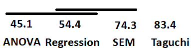
Two overlapping underlines are needed: one connecting ANOVA–Regression, and a second connecting Regression–SEM. ANOVA and SEM are significantly different from each other and cannot share an underline.

More precisely, with sample means 45.1 (ANOVA), 54.4 (Regression), 74.3 (SEM), 83.4 (Taguchi):

Tukey HSD Groupings

Technique	\(\bar{x}_i\)	Significantly different from
ANOVA	45.1	SEM, Taguchi; not from Regression
Regression	54.4	Taguchi; not from ANOVA or SEM
SEM	74.3	ANOVA, Taguchi; not from Regression
Taguchi	83.4	All others (ANOVA, Regression, SEM)

Conclusion: The Taguchi method has the highest mean effectiveness at the population level. It has the largest sample mean (\(\bar{x}_{\text{Taguchi}} = 83.4\)) and is statistically significantly different from all other techniques at the 5% family-wise error level.

—

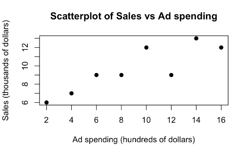
Problem 6 Setup

A marketing analyst studies the relationship between weekly online advertising spending (\(x\), in hundreds of dollars) and weekly sales (\(Y\), in thousands of dollars) over 8 weeks.

Advertising Spending and Sales Data

Variable	1	2	3	4	5	6	7	8
Ad spending (\(x\), hundreds $)	2	4	6	8	10	12	14	16
Sales (\(Y\), thousands $)	6	7	9	9	12	9	13	12

Summary statistics: \(\sum x_i = 72\), \(\sum x_i^2 = 816\), \(\sum y_i = 77\), \(\sum y_i^2 = 785\), \(\sum x_i y_i = 768\).

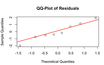
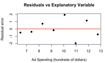
The scatter plot and regression diagnostics below were produced from the data.

Problem 6 — Simple Linear Regression (38 points)

Question 6a (10 pts)

Compute the least-squares regression line for predicting weekly sales from weekly advertising spending.

Solution

\(\bar{x} = 72/8 = 9\), \(\bar{y} = 77/8 = 9.625\).

\[S_{xy} = \sum x_i y_i - n\bar{x}\bar{y} = 768 - 8(9)(9.625) = 768 - 693 = 75\]

\[S_{xx} = \sum x_i^2 - n\bar{x}^2 = 816 - 8(9)^2 = 816 - 648 = 168\]

Slope:

\[b_1 = \frac{S_{xy}}{S_{xx}} = \frac{75}{168} = \boxed{0.4464}\]

Intercept:

\[b_0 = \bar{y} - b_1\bar{x} = 9.625 - 0.4464(9) = 9.625 - 4.0179 = \boxed{5.6071}\]

Fitted regression equation:

\[\hat{y} = 5.6071 + 0.4464\,x_{\text{Ad Spending}}\]

Interpretation of slope: For each additional $100 in weekly advertising spending, the estimated mean weekly sales increase by approximately $446.40 (i.e., 0.4464 thousand dollars).

Question 6b (7 pts)

Complete all missing entries in the ANOVA table below.

Regression ANOVA Table

Source	df	SS	MS	F	\(\Pr(>F)\)
Model	1	33.48	33.48	19.3336	0.0046
Error	6	10.39	1.7317
Total	7	43.87

Solution

Degrees of freedom: \(\text{df}_M = 1\), \(\text{df}_E = n - 2 = 6\), \(\text{df}_T = n - 1 = 7\).

SSR = \(b_1 \cdot S_{xy} = (75/168) \times 75 = 5625/168 \approx 33.48\).

SST = \(S_{yy} = \sum y_i^2 - n\bar{y}^2 = 785 - 8(9.625)^2 = 785 - 741.125 = 43.875 \approx 43.87\).

SSE = SST − SSR \(= 43.87 - 33.48 = 10.39\).

MSE = SSE / \(\text{df}_E = 10.39 / 6 = 1.7317\).

F = MSR / MSE \(= 33.48 / 1.7317 = 19.3336\). Cross-check: \(\Pr(>F) = 0.0046\).

Question 6c (4 pts)

Compute \(R^2\) and interpret it in context.

Solution

\[R^2 = \frac{\text{SSR}}{\text{SST}} = \frac{33.48}{43.87} = \boxed{0.7632}\]

Approximately 76.32% of the variation in weekly sales is explained by the linear relationship with weekly advertising spending.

Question 6d (4 pts)

Compute the Pearson correlation coefficient \(r\) and interpret it in context.

Solution

Since \(b_1 > 0\), the association is positive, so:

\[r = +\sqrt{R^2} = +\sqrt{0.7632} = \boxed{0.8736}\]

There is a strong positive linear association between weekly advertising spending and weekly sales. As ad spending increases, sales tend to increase as well.

Note on solution key ⚠️

The solution key correctly computes \(r = +\sqrt{0.7632} = 0.8736\), but then states in the interpretation sentence “r = 0.8580.” The value 0.8580 is incorrect; the correct value is 0.8736. The conclusion language uses 0.8736 in the box and 0.8580 in prose — follow the computed box value.

Question 6e (4 pts)

Compute \(s\), the estimate of \(\sigma\) (the standard deviation of the error terms).

Solution

\[s = \sqrt{\text{MSE}} = \sqrt{1.7317} = \boxed{1.3160}\]

Question 6f (4 pts)

To test \(H_0\colon \beta_1 = 0\) versus \(H_a\colon \beta_1 \neq 0\), what is the value of the \(t\)-test statistic?

Solution

For simple linear regression, \(F_{\text{TS}} = t_{\text{TS}}^2\). Since \(b_1 > 0\):

\[t_{\text{TS}} = +\sqrt{F_{\text{TS}}} = +\sqrt{19.3336} = \boxed{4.3970}\]

Degrees of freedom: \(\text{df}_E = n - 2 = 6\).

Question 6g (5 pts)

Is there a significant linear association between advertising spending and sales at \(\alpha = 0.01\)? State the hypotheses and provide a formal conclusion.

Solution

Step 1 — Parameter of interest: Let \(\beta_1\) be the true slope of the linear relationship between weekly advertising spending and weekly sales.

Step 2 — Hypotheses:

\[H_0\colon \beta_1 = 0 \quad \text{(no linear association between ad spending and sales)}\]

\[H_a\colon \beta_1 \neq 0 \quad \text{(there is a linear association)}\]

Step 3 — Test statistic and p-value:

\(F_{\text{TS}} = 19.3336\) on \(\text{df}_M = 1\), \(\text{df}_E = 6\); \(p\text{-value} = 0.0046\).

Step 4 — Decision and conclusion:

Since \(p\text{-value} = 0.0046 < 0.01 = \alpha\), we reject \(H_0\).

The data give support (\(p\)-value \(= 0.0046\)) to the claim that there is a linear association between weekly online advertising spending and weekly sales in the population.