3.2. Measures of Central Tendency

When analyzing data, one of the first questions we ask is: “What’s the typical value?” In this chapter, we’ll explore three fundamental measures of central tendency that can be used to answer this.

For simplicity, we will denote the variable under study as \(x\) throughout this section.

Road Map 🧭

• Define sample mode, sample mean, and sample median. Learn their mathematical notations and properties.

• Describe the strengths and weaknesses of each measure, and recognize which measure is the most appropriate given a data set.

3.2.1. Sample Mode, \(M\)

The sample mode is the simplest measure of central tendency—it’s the value that occurs most frequently in a dataset. We denote the sample mode with \(M\).

Properties

1. A data set might have zero, one, or more than one mode.

   • Zero when all values occur with equal frequency

   • One when exactly one value occurs most frequently

   • “Multimodal” when multiple values tie for the most frequent

   • A dataset with one mode is called unimodal. Datasets with two and three modes are called bimodal and trimodal, respectively.

2. The sample mode is most useful when working with discrete numerical data with a limited set of possible values.

3. It is less informative when the data contains many unique values with few repetitions. For this reason, the sample mode is not often used unless the data set is very simple.

Example 💡: Finding the Sample Mode

Consider this simple dataset: {1, 1, 2, 3, 4}

Since 1 occurs with the highest frequency, M = 1.

R doesn’t have a built-in function for computing the sample mode. Therefore, we need to create a new function.

# define a new function:
getmode <- function(v) {
   uniqv <- unique(v)
   uniqv[which.max(tabulate(match(v, uniqv)))]
   }

# define data
x <- c(1,1,2,3,4)

# use the newly defined function
getmode(x) # returns 1

Note: You may copy and paste the function above for your own use. If you’re interested in learning how to create your own functions, a general guide to defining custom R functions is provided in the appendix. However, you are not expected to write or define functions in this course.

3.2.2. Sample Mean, \(\bar{x}\)

The sample mean, denoted as \(\bar{x}\) (pronounced “x-bar”), is what most people think of as the “average.” The sample mean is calculated by summing all observations and dividing by the sample size:

\[\bar{x} = \frac{1}{n}\sum_{i=1}^{n} x_i = \frac{x_1 + x_2 + \ldots + x_n}{n}\]

Properties

1. It is influenced by each observation in the dataset.

2. It can be affected significantly by outliers or extreme values.

Example 💡: Finding the Sample Mean

For the dataset \(\{2, 4, 6, 8\}\),

\[\bar{x} = \frac{2 + 4 + 6 + 8}{4} = \frac{20}{4} = 5.\]

R provides a built-in function for calculating the mean.

x <- c(2, 4, 6, 8)
mean(x)  # Returns 5

3.2.3. Sample Median, \(\tilde{x}\)

The sample median, denoted as \(\tilde{x}\) (pronounced “x-tilde”), is the middle value when the data is arranged in order. It splits the dataset so that 50% of observations fall below and 50% fall above it.

How to find the sample median

1. Arrange all observations in ascending order.

2. If there is an odd number of observations, the median is the middle value.

3. If there is an even number of observations, the median is the average of the two middle values.

Mathematically,

\[\begin{split}\tilde{x} = \begin{cases} x_{\left(\frac{n+1}{2}\right)}, & \text{if } n \text{ is odd} \\[4pt] \frac{x_{\left(\frac{n}{2}\right)} + x_{\left(\frac{n}{2}+1\right)}}{2}, & \text{if } n \text{ is even} \end{cases}\end{split}\]

where \(x_{(i)}\) represents the \(i\)-th smallest value in the dataset.

Properties

1. It depends only on the order (ranks) of most of the data, not the exact values.

2. It is robust to outliers—extreme values don’t change it significantly.

Example 💡: Finding the sample median when \(n\) is odd

Take the data set \(\{1, 2, 4, 6, 8\}\). The data is already sorted with \(n = 5\).

\[\frac{n+1}{2} = \frac{5+1}{2} = 3.\]

The median is \(\tilde{x} = x_{(3)} = 4\).

y <- c(1, 2, 4, 6, 8)
median(y)  # Returns 4

Example 💡: Finding the sample median when \(n\) is even

The dataset \(\{2, 4, 6, 8\}\) has \(n=4\), which is even. \(\frac{n}{2} = \frac{4}{2} = 2\). The median is the average of the 2nd and 3rd values:

\[\tilde{x} = \frac{x_{(2)} + x_{(3)}}{2} = \frac{4 + 6}{2} = 5.\]

x <- c(2, 4, 6, 8)
median(x)  # Returns 5

3.2.4. Comparing the Measures: An Example

To better understand how the different measures of central tendency work in practice, let’s explore an example in depth.

Part 1

Miss Claridge asked her preschool class of nine students how many pets each had in their household. The results are recorded in the table below. A dot plot of the data is shown in Fig. 3.1.

Unsorted pet counts data
4	8	7	9	4	3	5	1	4

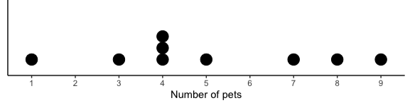
Fig. 3.1 Dot plot of pet counts

We will analyze this data using the three measures of central tendency. Let us begin by expressing the data using formal notion. Write the variable of pet counts with \(x\). We have \(n=9\). The individual data points are then denoted as \(x_1, x_2, \cdots, x_9\).

1. Sample Mode

   The value 4 occurs most frequently (three times). Therefore, \(M = 4\).

2. Sample Mean

   \[\bar{x} = \frac{1}{9}\sum_{i=1}^9 x_i = \frac{1}{9}(4 + 8 + 7 + 9 + 4 + 3 + 5 + 1 + 4) = \frac{45}{9} = 5\]

3. Sample Median

   First, sort the data: {1, 3, 4, 4, 4, 5, 7, 8, 9}. Since \(n\) is odd, compute \((9+1)/2 = 5\). The median is the 5th value. \(\tilde{x} = 4\).

Part 2

Miss Claridge discovers that there was an error during the data recording process: the student who was recorded as having nine pets actually had nineteen. How will the measures change due to this update?

New sorted pet counts data
1	3	4	4	4	5	7	8	9 → 19

1. Sample Mode

   The value 4 still occurs most frequently. \(M = 4\).

2. Sample Mean

   \[\bar{x} = \frac{1}{9}\sum_{i=1}^9 x_i = \frac{1}{9}(1+3+4+4+4+5+7+8+19) = \frac{55}{9} = 6.11\]

3. Sample Median

   \(n\) did not change. \((9+1)÷2 = 5\). The median is still the 5th value. \(\tilde{x} = 4\).

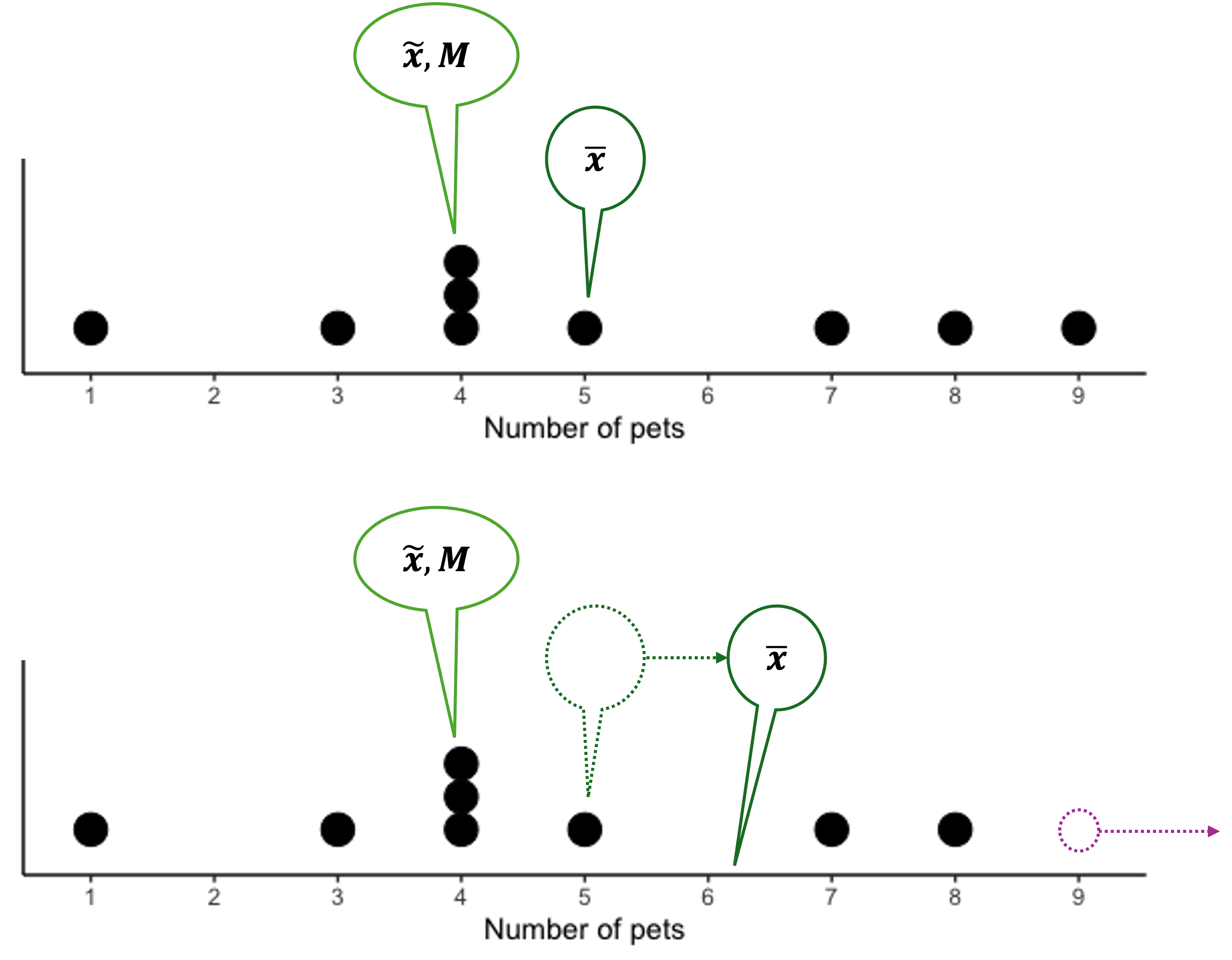
Fig. 3.2 Upper graph: central tendency measures before update. Lower: after update.

In Part 2, both the sample mode and median remained at 4, while the sample mean increased from 5 to 6.11. This illustrates how the sample mean is pulled towards all data points, including outliers and extreme values. In contrast, the sample median and mode are more resistant to such influences.

3.2.5. Bringing It All Together

Key Takeaways 📝

1. Measures of central tendency indicate where the majority of the data is centered, bunched, or clustered.

2. The sample mode (\(M\)) finds the most frequent value(s) and works best for discrete data with few unique values.

3. The sample mean (\(\bar{x}\)) calculates the arithmetic average. It’s sensitive to outliers but works well for symmetric distributions.

4. The sample median (\(\tilde{x}\)) finds the middle value and is robust against extreme values. It’s often better than the mean for skewed distributions.

5. The three measures do not always tell the same story. Choose the most appropriate measure by understanding the data’s charateristics.

Exercises

1. For each scenario below, indicate which measure of central tendency (mode, mean, or median) would be most appropriate and explain why:

   1. Annual income in a small town with a few extremely wealthy residents

   2. Most common shirt size sold in a clothing store

   3. Average test score in a normally distributed exam

2. Consider the dataset {2, 2, 3, 4, 5, 5, 5, 6, 10, 15}:

   1. Calculate the mode, mean, and median.

   2. Create a dot plot and mark each measure.

   3. Explain why the measures differ.

   4. If the value 15 were changed to 50, recalculate all three measures. Which one changed the most? Which changed the least? Explain why.

3. Challenge Problem: A teacher gives two exams to the same class. The mean score is the same on both exams, but the median is higher on the second exam. What does this tell you about how the distribution of scores changed from the first exam to the second?

Appendix: Defining Your Own Functions in R

As we’ve seen with our sample mode function, R allows us to create custom functions for statistical operations that aren’t built into the language. The basic structure of a function in R is:

function_name <- function(argument1, argument2, ...) {
  # Code goes between brackets
  return(return_value) # Can return a single entity
}

Let’s break down the components:

• Function name: The name you’ll use when calling the function

• Arguments: The list of input values

  • Arguments can have default values: function(argument = 0)

  • You can create functions with no arguments: function()

• Function body (Everything between the curly brackets { }): code describing the steps to be taken when the function is called

• Return value: What the function outputs after computation