Slides 📊

Download Chapter 6 slides (PPTX)

6.6. Exponential Distribution

We now encounter the exponential distribution, which captures the essence of decay and waiting times.

Road Map 🧭

• Understand the exponential distribution as a model for waiting times between events.

• Distinguish between Poisson (counting events) and exponential (measuring length of time between events) distributions.

• Master the exponential PDF and CDF.

• Explore the memoryless property of exponential random variables.

• Learn about the two ways of parameterizing an exponential distribution: using the rate parameter \(\lambda\) vs. the mean parameter \(\mu\).

6.6.1. From Event Counting to Waiting Times

Consider a hospital emergency room where patients arrive according to a Poisson process with an average rate of 3 patients per hour. The Poisson distribution tells us the probabilities of seeing 0, 1, 2, or more patients in any given hour. But suppose we ask instead: “Given that a patient has just arrived, how long will it be until the next one arrives?”

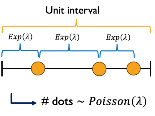
This waiting time follows an exponential distribution. The connection is profound: if events occur according to a Poisson process with rate \(\lambda\), then the time between consecutive events follows an exponential distribution with the same rate parameter \(\lambda\).

Why “Exponential”?

The distribution gets its name from the patterns in its probability density function. It assigns the highest probability density to small wait times and exponentially decreasing density to higher wait times. This reflects an intuitive property of many real-world processes—short wait times are much more likely than long wait times, but extremely long wait times, while rare, remain possible.

6.6.2. Mathematical Definition and Properties

The Exponential PDF

A continuous random variable \(X\) follows an exponential distribution if its probability density function is:

\[\begin{split}f_X(x) = \begin{cases} \lambda e^{-\lambda x} & \text{for } x \geq 0 \\ 0 & \text{for } x < 0 \end{cases}\end{split}\]

We write \(X \sim \text{Exp}(\lambda)\) or \(X \sim \text{Exponential}(\lambda)\).

Understanding the Components

• Rate parameter \(\lambda\): Just like in Poisson distributions, \(\lambda\) represents the average number of events per unit time and is therefore always positive. Higher values of \(\lambda\) indicate more frequent events which lead to shorter expected waiting times.

• Exponential decay \(e^{-\lambda x}\) creates the characteristic decreasing curve.

• \(\text{supp}(X) =[0, \infty)\) because waiting times cannot be negative.

• The PDF starts at its maximum value \(\lambda\) when \(x = 0\) and decreases exponentially, approaching but never reaching zero as \(x \to \infty\).

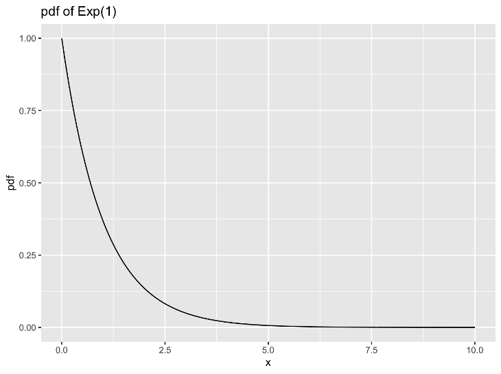
Fig. 6.53 An exponential PDF

The Expoenential CDF

The cumulative distribution function requires integrating the PDF. For any \(x \geq 0\),

\[\begin{split}F_X(x) &= P(X \leq x) = \int_0^x \lambda e^{-\lambda s} \, ds = \lambda \left[ \frac{e^{-\lambda s}}{-\lambda} \right]_0^x\\ &= \lambda \left[ \frac{e^{-\lambda x} - e^0}{-\lambda} \right] = \lambda \left[ \frac{e^{-\lambda x} - 1}{-\lambda} \right] = 1 - e^{-\lambda x}\end{split}\]

Therefore, the exponential CDF is:

\[\begin{split}F_X(x) = \begin{cases} 1 - e^{-\lambda x} & \text{for } x \geq 0 \\ 0 & \text{for } x < 0 \end{cases}\end{split}\]

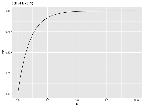
Fig. 6.54 An exponential CDF

A Notable Property

The exponential CDF approaches 1 as \(x \to \infty\), but technically only equals 1 in the limit. This occurs because the PDF never actually reaches zero on the right tail.

6.6.3. Expected Value and Variance

Expected Value

To find \(E[X]\), we compute:

\[E[X] = \int_0^{\infty} x \cdot \lambda e^{-\lambda x} \, dx\]

This requires integration by parts with \(u = x\) and \(dv = \lambda e^{-\lambda x} dx\):

• \(du = dx\)

• \(v = -e^{-\lambda x}\)

\[E[X] = \left[ x (-e^{-\lambda x}) \right]_0^{\infty} - \int_0^{\infty} (-e^{-\lambda x}) \, dx\]

The first term equals zero since \(xe^{-\lambda x} \to 0\) as \(x \to \infty\) and \(x(-e^{-\lambda x})=0\) at \(x = 0\), leaving:

\[E[X] = \int_0^{\infty} e^{-\lambda x} \, dx = \left[ \frac{e^{-\lambda x}}{-\lambda} \right]_0^{\infty} = \frac{1}{\lambda}.\]

Variance

For variance, we use \(\text{Var}(X) = E[X^2] - (E[X])^2\). Finding \(E[X^2]\) requires another integration by parts, which we leave as an independent exercise.

\[E[X^2] = \int_0^{\infty} x^2 \cdot \lambda e^{-\lambda x} \, dx = \frac{2}{\lambda^2}\]

Therefore,

\[\text{Var}(X) = E[X^2] - (E[X])^2 = \frac{2}{\lambda^2} - \left(\frac{1}{\lambda}\right)^2 = \frac{2}{\lambda^2} - \frac{1}{\lambda^2} = \frac{1}{\lambda^2}.\]

Summary

For \(X \sim \text{Exp}(\lambda)\),

\[E[X] = \frac{1}{\lambda} \quad \text{and} \quad \text{Var}(X) = \frac{1}{\lambda^2}.\]

The standard deviation is \(\sigma_X = \frac{1}{\lambda}\).

Interpretation

If events occur at the rate \(\lambda\) per unit time, we expect to wait \(\frac{1}{\lambda}\) time units on average until the next event. Higher rates mean shorter waiting times, and the variance decreases as the rate increases, indicating more predictable waiting times.

6.6.4. Two Parameterizations: Rate vs. Mean

The exponential distribution can be parameterized in two equivalent ways, each emphasizing different aspects of the underlying process.

Rate Parameterization

The rate parameterization uses \(\lambda > 0\) as we’ve seen:

\[f_X(x) = \lambda e^{-\lambda x}, \quad x \geq 0\]

Here, \(\lambda\) represents the average number of events per unit time. This parameterization is natural when we think about process rates: phone calls per minute, component failures per year, or customer arrivals per hour.

Mean Parameterization

The mean parameterization uses \(\mu = \frac{1}{\lambda}\) as the parameter:

\[f_X(x) = \frac{1}{\mu} e^{-x/\mu}, \quad x \geq 0\]

Here, \(\mu\) represents the average waiting time between events. This parameterization is natural when we think about typical waiting times: average time between phone calls, mean component lifetime, or expected time between customer arrivals.

Converting Between Parameterizations

The relationship \(\mu = \frac{1}{\lambda}\) allows easy conversion:

• If events occur at rate \(\lambda = 3\) per hour, the mean waiting time is \(\mu = \frac{1}{3}\) hour (20 minutes).

• If the mean waiting time is \(\mu = 2\) minutes, the rate is \(\lambda = \frac{1}{2}\) events per minute (30 events per hour).

Choosing the Right Parameterization

Use the parameterization that matches your problem’s natural description.

• Use rate parameterization when the problem gives or asks for rates (“failures per year”, “arrivals per hour”).

• Use mean parameterization when the problem gives or asks for typical waiting times (“mean time to failure”, “average service time”).

6.6.5. The Memoryless Property

For any exponential random variable \(X\) and any positive values \(s\) and \(t\):

\[P(X > s + t \mid X > s) = P(X > t)\]

The memoryless property implies that if we’ve already waited time \(s\) without an event occurring, the probability of waiting an additional time \(t\) is the same as if we were starting fresh. The process “forgets” how long we’ve already waited—past waiting time provides no information about future waiting time.

Proving the Memoryless Property

Using the definition of conditional probability,

\[P(X > s + t \mid X > s) = \frac{P(\{X > s + t\} \cap \{X > s\})}{P(X > s)} = \frac{P(X > s + t)}{P(X > s)}\]

From the exponential CDF \(F_X(x) = 1 - e^{-\lambda x}\), we get \(P(X > x) = e^{-\lambda x}\). Using this,

\[P(X > s + t \mid X > s) = \frac{e^{-\lambda(s+t)}}{e^{-\lambda s}} = \frac{e^{-\lambda s} \cdot e^{-\lambda t}}{e^{-\lambda s}} = e^{-\lambda t} = P(X > t)✔\]

Example💡: Exponential Distribution

Customers arrive at a service desk with exponentially distributed inter-arrival times averaging 4 minutes.

1. What’s the probability that no customer arrives for the next 2 minutes?

   Let \(Y\) denote the inter-arrival wait time. \(Y \sim \text{Exp}(\mu=4)\). The parameter is provided as an average time, so we use \(\mu\).

   \[P(Y > 2) = 1 - F_Y(y) = 1 - (1 - e^{-2/4}) = e^{-2/4} = 0.6065\]

2. If no customer has arrived in the last 6 minutes, what’s the probability one arrives in the next minute?

   Begin by setting up the probability statement. We are looking for \(P(Y < 6 + 1 | Y > 6)\). Using memoryless property of exponential \(Y\), this is equal to \(P(Y < 1)\).

   \[P(Y < 1) = 1 - e^{-1/4} = 0.2212\]

3. Find the time \(t\) such that 90% of inter-arrival times are less than \(t\).

   We need to find \(t\) such that \(F_Y(t) = P(Y \leq t) = 0.9\). Replacing the left-hand side with the CDF of \(Y\) and solving for \(t\),

   \[1 - e^{-t/4} = 0.9 \implies t = -4\cdot\text{ln}(0.1)=9.21.\]

   90% of the wait times at this service desk fall on or below 9.21 minutes.

6.6.6. Summary: Properties of Exponential Distribution

• Notation: \(X \sim \text{Exp}(\lambda)\) or \(X \sim \text{Exponential}(\lambda)\)

• Parameter: \(\lambda > 0\) (rate parameter) or \(\mu = \frac{1}{\lambda} > 0\) (mean parameter)

• Support: \([0, \infty)\)

• PDF: \(f_X(x) = \begin{cases} \lambda e^{-\lambda x} & \text{for } x \geq 0 \\ 0 & \text{for } x < 0 \end{cases}\)

• CDF: \(F_X(x) = \begin{cases} 1 - e^{-\lambda x} & \text{for } x \geq 0 \\ 0 & \text{for } x < 0 \end{cases}\)

• Expected Value: \(E[X] = \frac{1}{\lambda}\)

• Variance: \(\text{Var}(X) = \frac{1}{\lambda^2}\)

• Standard Deviation: \(\sigma_X = \frac{1}{\lambda}\)

• Memoryless Property: \(P(X > s + t \mid X > s) = P(X > t)\) for all \(s, t > 0\)

Distinguishing Between Poisson and Exponential Random Variables

This relationship often causes confusion, so let’s go through the differences explicitly:

Aspect	Poisson Distribution	Exponential Distribution
What does it describe?	# events per unit	Time until the next event
Discrete or continuous?	Discrete with support \(\{0, 1, 2, \cdots\}\)	Continuous with support \([0, \infty)\)
Parameter	\(\lambda\) = average number of events per unit time
Typical question	What is the probability that 3 customers arrive in the next hour?	What is the probability that no customer arrives for the next 40 minutes?

6.6.7. Bringing It All Together

Key Takeaways 📝

1. The exponential distribution models waiting times between events in a Poisson process. If events occur according to a Poisson process with rate \(\lambda\), then their inter-arrival times follow \(\text{Exp}(\lambda)\).

2. The PDF \(f_X(x) = \lambda e^{-\lambda x}, x \geq 0\) creates an exponential decay pattern.

3. The CDF is \(F_X(x) = 1 - e^{-\lambda x} , x \geq 0\).

4. Two parameterizations exist: one using the rate \(\lambda\) (events per time) and the other using the mean \(\mu = \frac{1}{\lambda}\) (average waiting time).

5. The memoryless property \(P(X > s + t \mid X > s) = P(X > t)\) uniquely characterizes exponential distributions among continuous distributions.

6.6.8. Exercises

These exercises develop your skills in working with exponential distributions, including computing probabilities using the PDF and CDF, converting between rate and mean parameterizations, applying the memoryless property, and understanding the connection to Poisson processes.

Key Formulas

For \(X \sim \text{Exp}(\lambda)\) where \(\lambda\) is the rate parameter:

• PDF: \(f_X(x) = \lambda e^{-\lambda x}\) for \(x \geq 0\)

• CDF: \(F_X(x) = 1 - e^{-\lambda x}\) for \(x \geq 0\)

• Survival Function: \(P(X > x) = e^{-\lambda x}\)

• Expected Value: \(E[X] = \frac{1}{\lambda}\) (mean waiting time)

• Variance: \(\text{Var}(X) = \frac{1}{\lambda^2}\)

• Standard Deviation: \(\sigma_X = \frac{1}{\lambda}\) (uniquely for exponential distributions, SD = mean)

• Memoryless Property: \(P(X > s + t \mid X > s) = P(X > t)\)

Parameterization Note

The exponential distribution can be parameterized by rate \(\lambda\) (events per unit time) or by mean \(\mu = \frac{1}{\lambda}\) (average waiting time). With mean parameterization: \(f_X(x) = \frac{1}{\mu} e^{-x/\mu}\) and \(F_X(x) = 1 - e^{-x/\mu}\).

Exercise 1: Basic Exponential Calculations

Server response times at a data center follow an exponential distribution with rate \(\lambda = 0.5\) responses per second.

1. Write out the PDF \(f_X(x)\) and CDF \(F_X(x)\).

2. Find \(P(X \leq 2)\) — the probability a response takes at most 2 seconds.

3. Find \(P(X > 3)\) — the probability a response takes more than 3 seconds.

4. Find \(P(1 < X < 4)\) — the probability a response takes between 1 and 4 seconds.

5. Sketch the PDF and indicate the region corresponding to part (d).

Solution

Let \(X\) = server response time (seconds), where \(X \sim \text{Exp}(\lambda = 0.5)\).

Part (a): PDF and CDF

\[\begin{split}f_X(x) = \begin{cases} 0.5 e^{-0.5x} & \text{for } x \geq 0 \\ 0 & \text{for } x < 0 \end{cases}\end{split}\]

\[\begin{split}F_X(x) = \begin{cases} 1 - e^{-0.5x} & \text{for } x \geq 0 \\ 0 & \text{for } x < 0 \end{cases}\end{split}\]

Part (b): P(X ≤ 2)

\[P(X \leq 2) = F_X(2) = 1 - e^{-0.5(2)} = 1 - e^{-1} = 1 - 0.3679 = 0.6321\]

Part (c): P(X > 3)

Using the survival function:

\[P(X > 3) = e^{-0.5(3)} = e^{-1.5} = 0.2231\]

Or equivalently: \(P(X > 3) = 1 - F_X(3) = 1 - (1 - e^{-1.5}) = e^{-1.5} = 0.2231\).

Part (d): P(1 < X < 4)

\[P(1 < X < 4) = F_X(4) - F_X(1) = (1 - e^{-2}) - (1 - e^{-0.5}) = e^{-0.5} - e^{-2}\]

\[= 0.6065 - 0.1353 = 0.4712\]

Part (e): PDF sketch

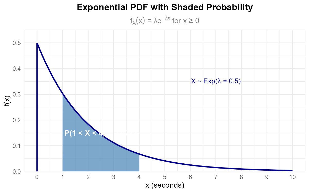
Fig. 6.55 The exponential PDF with P(1 < X < 4) = 0.4712 shaded.

---

Exercise 2: Expected Value and Variance

The time between arrivals at an emergency room follows an exponential distribution with rate \(\lambda = 4\) patients per hour.

1. Find the expected time between arrivals (in minutes).

2. Find the variance and standard deviation of the time between arrivals.

3. What is notable about the relationship between the mean and standard deviation for exponential distributions?

4. If the arrival rate doubled to 8 patients per hour, how would the expected waiting time change?

Solution

Let \(X\) = time between arrivals (hours), where \(X \sim \text{Exp}(\lambda = 4)\).

Part (a): Expected time between arrivals

\[E[X] = \frac{1}{\lambda} = \frac{1}{4} \text{ hour} = 15 \text{ minutes}\]

Part (b): Variance and standard deviation

\[\text{Var}(X) = \frac{1}{\lambda^2} = \frac{1}{16} \text{ hours}^2\]

\[\sigma_X = \frac{1}{\lambda} = \frac{1}{4} \text{ hour} = 15 \text{ minutes}\]

Part (c): Mean equals standard deviation

For exponential distributions, \(E[X] = \sigma_X = \frac{1}{\lambda}\). This equality is a unique property of the exponential distribution—it does not hold for other continuous distributions. It reflects the high variability inherent in exponential waiting times: the coefficient of variation (CV = σ/μ) is always exactly 1.

Part (d): Effect of doubling the rate

If \(\lambda = 8\) patients per hour:

\[E[X] = \frac{1}{8} \text{ hour} = 7.5 \text{ minutes}\]

Doubling the arrival rate halves the expected waiting time. This inverse relationship is characteristic of exponential distributions.

---

Exercise 3: Rate vs. Mean Parameterization

Convert between parameterizations and express the PDF in both forms.

1. A machine’s time to failure has rate \(\lambda = 0.02\) failures per day. Express this using the mean parameterization and find \(E[X]\).

2. A call center has an average call duration of \(\mu = 6\) minutes. Express this using the rate parameterization and write the PDF.

3. Network packets arrive with a mean inter-arrival time of 50 milliseconds. Find the rate parameter and calculate \(P(X > 75)\).

4. If \(\lambda = 1.5\) events per hour, find \(P(X \leq 30 \text{ minutes})\).

Solution

Part (a): Rate to mean parameterization

Given \(\lambda = 0.02\) failures per day:

\[\mu = \frac{1}{\lambda} = \frac{1}{0.02} = 50 \text{ days}\]

Mean parameterization: \(X \sim \text{Exp}(\mu = 50)\) where \(\mu\) is mean time to failure.

PDF: \(f_X(x) = \frac{1}{50} e^{-x/50}\) for \(x \geq 0\).

Expected value: \(E[X] = \mu = 50\) days.

Part (b): Mean to rate parameterization

Given \(\mu = 6\) minutes:

\[\lambda = \frac{1}{\mu} = \frac{1}{6} \text{ calls per minute}\]

Rate parameterization: \(X \sim \text{Exp}(\lambda = \frac{1}{6})\).

PDF: \(f_X(x) = \frac{1}{6} e^{-x/6}\) for \(x \geq 0\).

Part (c): Mean inter-arrival time to probability

Given \(\mu = 50\) ms, so \(\lambda = \frac{1}{50} = 0.02\) packets per ms.

\[P(X > 75) = e^{-\lambda \cdot 75} = e^{-0.02 \times 75} = e^{-1.5} = 0.2231\]

Alternatively, using mean parameterization directly:

\[P(X > 75) = e^{-75/50} = e^{-1.5} = 0.2231\]

Part (d): Rate with unit conversion

Given \(\lambda = 1.5\) events per hour. For 30 minutes = 0.5 hours:

\[P(X \leq 0.5) = 1 - e^{-1.5 \times 0.5} = 1 - e^{-0.75} = 1 - 0.4724 = 0.5276\]

Alternatively, convert rate to per-minute: \(\lambda = \frac{1.5}{60} = 0.025\) per minute.

\[P(X \leq 30) = 1 - e^{-0.025 \times 30} = 1 - e^{-0.75} = 0.5276\]

---

Exercise 4: The Memoryless Property

A light bulb’s lifetime follows an exponential distribution with mean \(\mu = 1000\) hours.

1. Find the probability that a new bulb lasts more than 500 hours.

2. Given that a bulb has already lasted 800 hours, find the probability it lasts at least 300 more hours.

3. Verify that your answers to (a) and (b) demonstrate the memoryless property.

4. Given that a bulb has lasted 1500 hours, what is the expected additional lifetime?

5. Explain why the memoryless property might seem counterintuitive for light bulbs but is mathematically consistent.

Solution

Let \(X\) = bulb lifetime (hours), where \(X \sim \text{Exp}(\mu = 1000)\), so \(\lambda = \frac{1}{1000} = 0.001\).

Part (a): P(X > 500) for a new bulb

\[P(X > 500) = e^{-500/1000} = e^{-0.5} = 0.6065\]

Part (b): P(X > 1100 | X > 800) — conditional probability

We want \(P(X > 800 + 300 \mid X > 800)\).

By the memoryless property: \(P(X > s + t \mid X > s) = P(X > t)\).

\[P(X > 800 + 300 \mid X > 800) = P(X > 300) = e^{-300/1000} = e^{-0.3} = 0.7408\]

Part (c): Verify memoryless property

Let’s compute \(P(X > 300)\) directly:

\[P(X > 300) = e^{-300/1000} = e^{-0.3} = 0.7408\]

This matches part (b), confirming the memoryless property: the probability of surviving an additional 300 hours is the same whether the bulb is new or has already operated for 800 hours.

Part (d): Expected additional lifetime after 1500 hours

By the memoryless property, given that the bulb has survived to time \(s\), its remaining lifetime has the same distribution as a new bulb. Therefore:

\[E[X - 1500 \mid X > 1500] = E[X] = \mu = 1000 \text{ hours}\]

Even after 1500 hours of operation, the bulb “expects” to last another 1000 hours on average—exactly the same as a brand new bulb.

Part (e): Intuitive explanation

The memoryless property seems counterintuitive because physical light bulbs do wear out—their filaments degrade, making older bulbs more likely to fail. Real light bulb lifetimes are better modeled by Weibull or log-normal distributions.

However, the memoryless property is mathematically consistent for idealized processes where failure occurs due to random shocks (not wear). It’s appropriate for modeling radioactive decay, random equipment failures due to external factors, or certain types of electronic components.

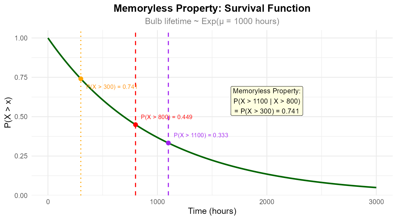
Fig. 6.56 The memoryless property: conditional survival probabilities equal unconditional probabilities.

---

Exercise 5: Finding Percentiles

Download times for a software update follow an exponential distribution with rate \(\lambda = 0.1\) per minute.

1. Find the median download time.

2. Find the 90th percentile of download times.

3. Find the time by which 25% of downloads are complete.

4. What proportion of downloads take longer than twice the mean?

Solution

Let \(X\) = download time (minutes), where \(X \sim \text{Exp}(\lambda = 0.1)\).

First note: \(E[X] = \frac{1}{0.1} = 10\) minutes.

Part (a): Median (50th percentile)

Find \(x_{0.50}\) such that \(F_X(x_{0.50}) = 0.50\):

\[1 - e^{-0.1 x_{0.50}} = 0.50\]

\[e^{-0.1 x_{0.50}} = 0.50\]

\[-0.1 x_{0.50} = \ln(0.50) = -0.6931\]

\[x_{0.50} = \frac{0.6931}{0.1} = 6.931 \text{ minutes}\]

Note: The median (6.93 min) is less than the mean (10 min) because exponential distributions are right-skewed.

Part (b): 90th percentile

Find \(x_{0.90}\) such that \(F_X(x_{0.90}) = 0.90\):

\[1 - e^{-0.1 x_{0.90}} = 0.90\]

\[e^{-0.1 x_{0.90}} = 0.10\]

\[x_{0.90} = \frac{-\ln(0.10)}{0.1} = \frac{2.303}{0.1} = 23.03 \text{ minutes}\]

90% of downloads complete within 23.03 minutes.

Part (c): 25th percentile

\[e^{-0.1 x_{0.25}} = 0.75\]

\[x_{0.25} = \frac{-\ln(0.75)}{0.1} = \frac{0.2877}{0.1} = 2.877 \text{ minutes}\]

25% of downloads complete within about 2.88 minutes.

Part (d): P(X > 2μ) = P(X > 20)

\[P(X > 20) = e^{-0.1 \times 20} = e^{-2} = 0.1353\]

About 13.5% of downloads take longer than twice the mean. This is a fixed property of all exponential distributions: \(P(X > 2\mu) = e^{-2} \approx 0.135\).

---

Exercise 6: Connection to Poisson Process

Customers arrive at a coffee shop according to a Poisson process with rate \(\lambda = 12\) customers per hour.

1. What is the distribution of the time between consecutive customer arrivals?

2. Find the probability that the time between two consecutive arrivals exceeds 10 minutes.

3. Find the expected time between arrivals.

4. If 5 minutes have passed since the last customer, what is the probability that the next customer arrives within the next 3 minutes?

5. In a given hour, what is the probability that exactly 10 customers arrive? (This uses the Poisson distribution.)

Solution

Part (a): Distribution of inter-arrival times

If arrivals follow a Poisson process with rate \(\lambda\), then the time between arrivals follows an exponential distribution with the same rate parameter.

\(X \sim \text{Exp}(\lambda = 12)\) where X is measured in hours.

Or equivalently: \(X \sim \text{Exp}(\lambda = 0.2)\) per minute (converting 12/hour to 12/60 = 0.2/minute).

Part (b): P(X > 10 minutes)

Using \(\lambda = 0.2\) per minute:

\[P(X > 10) = e^{-0.2 \times 10} = e^{-2} = 0.1353\]

Or using \(\lambda = 12\) per hour with 10 min = 1/6 hour:

\[P(X > 1/6) = e^{-12 \times (1/6)} = e^{-2} = 0.1353\]

Part (c): Expected time between arrivals

\[E[X] = \frac{1}{\lambda} = \frac{1}{12} \text{ hour} = 5 \text{ minutes}\]

Part (d): Conditional probability (memoryless property)

We want \(P(X \leq 8 \mid X > 5)\) where X is in minutes.

By the memoryless property:

\[P(X \leq 5 + 3 \mid X > 5) = P(X \leq 3)\]

\[P(X \leq 3) = 1 - e^{-0.2 \times 3} = 1 - e^{-0.6} = 1 - 0.5488 = 0.4512\]

Part (e): Poisson probability for counts

The number of arrivals in one hour follows \(N \sim \text{Poisson}(\lambda = 12)\).

\[P(N = 10) = \frac{e^{-12} \cdot 12^{10}}{10!} = \frac{e^{-12} \cdot 61917364224}{3628800} = 0.1048\]

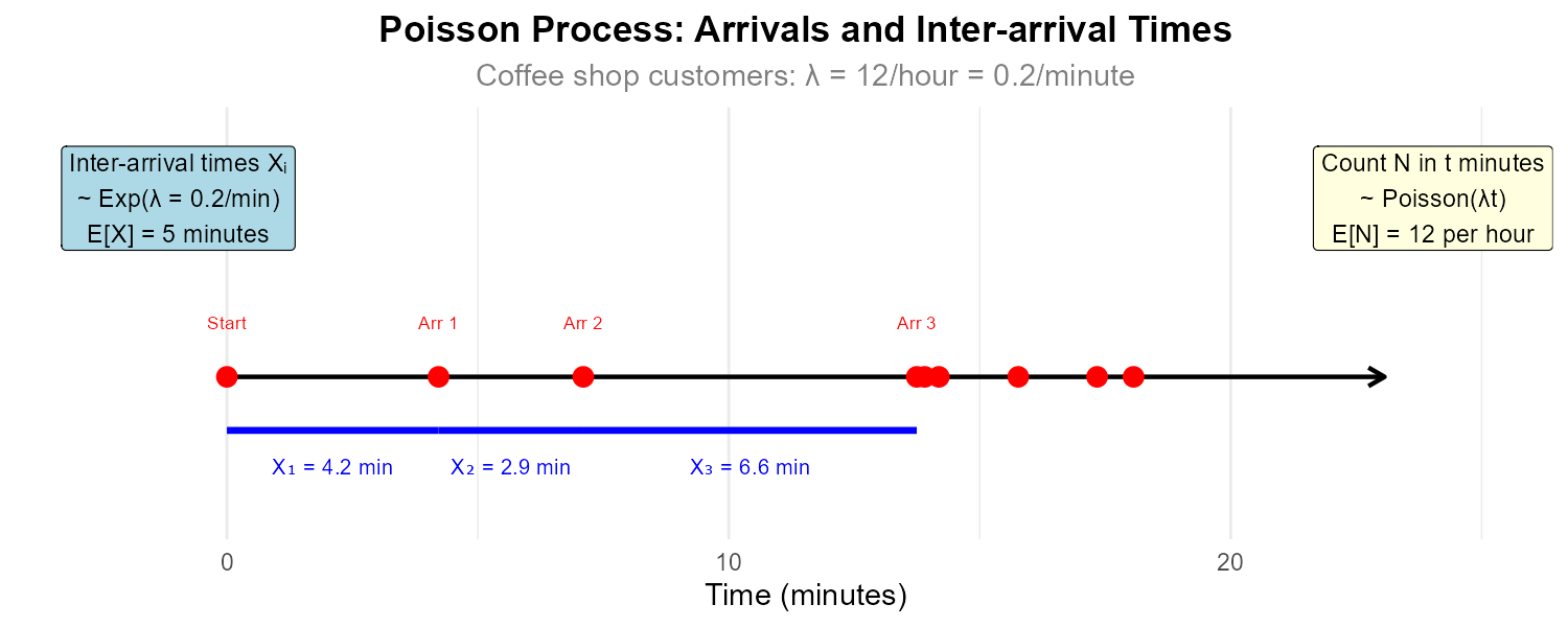
Fig. 6.57 The Poisson process: counts follow Poisson, inter-arrival times follow Exponential.

---

Exercise 7: Comparing Exponential Distributions

Two servers process requests. Server A has response times following \(\text{Exp}(\lambda_A = 2)\) per second, while Server B has response times following \(\text{Exp}(\lambda_B = 0.5)\) per second.

1. Which server has faster average response times? By how much?

2. For each server, find the probability that a response takes less than 1 second.

3. For each server, find the 95th percentile of response times.

4. Which server has more consistent (less variable) response times? Justify your answer.

Solution

Server A: \(X_A \sim \text{Exp}(\lambda = 2)\) per second.

Server B: \(X_B \sim \text{Exp}(\lambda = 0.5)\) per second.

Part (a): Expected response times

\[E[X_A] = \frac{1}{2} = 0.5 \text{ seconds}\]

\[E[X_B] = \frac{1}{0.5} = 2 \text{ seconds}\]

Server A is faster with average response time of 0.5 seconds compared to Server B’s 2 seconds. Server A is 4 times faster on average.

Part (b): P(X < 1 second)

Server A:

\[P(X_A < 1) = 1 - e^{-2 \times 1} = 1 - e^{-2} = 1 - 0.1353 = 0.8647\]

Server B:

\[P(X_B < 1) = 1 - e^{-0.5 \times 1} = 1 - e^{-0.5} = 1 - 0.6065 = 0.3935\]

Server A has 86.5% of responses under 1 second; Server B has only 39.4%.

Part (c): 95th percentile

For \(x_{0.95}\): \(e^{-\lambda x_{0.95}} = 0.05\), so \(x_{0.95} = \frac{-\ln(0.05)}{\lambda} = \frac{2.996}{\lambda}\).

Server A:

\[x_{0.95} = \frac{2.996}{2} = 1.498 \text{ seconds}\]

Server B:

\[x_{0.95} = \frac{2.996}{0.5} = 5.991 \text{ seconds}\]

95% of Server A’s responses complete within 1.5 seconds; for Server B, it’s 6 seconds.

Part (d): Variability comparison

\[\sigma_A = \frac{1}{\lambda_A} = 0.5 \text{ seconds}\]

\[\sigma_B = \frac{1}{\lambda_B} = 2 \text{ seconds}\]

Server A has more consistent response times (σ = 0.5 sec vs. σ = 2 sec).

Note: For exponential distributions, faster servers (higher λ) are always more consistent because both mean and standard deviation equal \(\frac{1}{\lambda}\).

---

Exercise 8: PDF and CDF Verification

Let \(X \sim \text{Exp}(\lambda)\).

1. Verify that \(f_X(x) = \lambda e^{-\lambda x}\) integrates to 1 over the support.

2. Verify that \(F_X(x) = 1 - e^{-\lambda x}\) is the antiderivative of \(f_X(x)\).

3. Find \(f_X(0)\) (the PDF at x = 0). What does this tell you about small waiting times?

4. Show that \(\lim_{x \to \infty} f_X(x) = 0\).

5. At what value of \(x\) does the PDF equal half its maximum value?

Solution

Part (a): Verify PDF integrates to 1

\[\int_0^{\infty} \lambda e^{-\lambda x} \, dx = \lambda \left[ \frac{e^{-\lambda x}}{-\lambda} \right]_0^{\infty} = -\left[ e^{-\lambda x} \right]_0^{\infty}\]

\[= -(e^{-\infty} - e^0) = -(0 - 1) = 1 \quad \checkmark\]

Part (b): Verify CDF is antiderivative of PDF

\[\frac{d}{dx} F_X(x) = \frac{d}{dx} (1 - e^{-\lambda x}) = 0 - (-\lambda) e^{-\lambda x} = \lambda e^{-\lambda x} = f_X(x) \quad \checkmark\]

Part (c): PDF at x = 0

\[f_X(0) = \lambda e^{-\lambda \cdot 0} = \lambda e^0 = \lambda\]

The PDF achieves its maximum value at x = 0. This means the highest probability density is assigned to very small waiting times—short waits are most likely. The larger λ is, the higher the density at 0 and the more concentrated probability is near small values.

Part (d): Limit as x → ∞

\[\lim_{x \to \infty} f_X(x) = \lim_{x \to \infty} \lambda e^{-\lambda x} = \lambda \cdot 0 = 0\]

The PDF approaches 0 asymptotically, meaning very long waiting times are increasingly rare but never impossible.

Part (e): Half-maximum point

The maximum is \(f_X(0) = \lambda\). We want \(f_X(x) = \frac{\lambda}{2}\):

\[\lambda e^{-\lambda x} = \frac{\lambda}{2}\]

\[e^{-\lambda x} = \frac{1}{2}\]

\[-\lambda x = \ln(0.5) = -\ln(2)\]

\[x = \frac{\ln(2)}{\lambda} = \frac{0.693}{\lambda}\]

This is exactly the median of the distribution. This coincidence—that the PDF drops to half its maximum at the median—is a special property of the exponential distribution and does not hold for other distributions.

---

Exercise 9: Application — System Reliability

A critical sensor has a lifetime that follows an exponential distribution with mean 2 years. The sensor must be replaced when it fails.

1. Find the probability that a new sensor lasts at least 3 years.

2. Find the probability that a sensor fails within the first 6 months.

3. The manufacturer offers a 1-year warranty. What proportion of sensors will fail under warranty?

4. A sensor has been operating for 18 months without failure. What is the probability it lasts at least another year?

5. If 100 identical sensors are deployed, how many are expected to fail within the first year?

6. Find the time by which 80% of sensors are expected to have failed.

Solution

Let \(X\) = sensor lifetime (years), where \(X \sim \text{Exp}(\mu = 2)\), so \(\lambda = \frac{1}{2} = 0.5\) per year.

Part (a): P(X ≥ 3)

\[P(X \geq 3) = e^{-0.5 \times 3} = e^{-1.5} = 0.2231\]

About 22.3% of sensors last at least 3 years.

Part (b): P(X ≤ 0.5) — failure within 6 months

\[P(X \leq 0.5) = 1 - e^{-0.5 \times 0.5} = 1 - e^{-0.25} = 1 - 0.7788 = 0.2212\]

About 22.1% fail within the first 6 months.

Part (c): P(X ≤ 1) — warranty claims

\[P(X \leq 1) = 1 - e^{-0.5 \times 1} = 1 - e^{-0.5} = 1 - 0.6065 = 0.3935\]

About 39.4% of sensors will fail under the 1-year warranty.

Part (d): Conditional probability (memoryless)

After 18 months (1.5 years), what is P(X > 2.5 | X > 1.5)?

By the memoryless property:

\[P(X > 1.5 + 1 \mid X > 1.5) = P(X > 1) = e^{-0.5 \times 1} = e^{-0.5} = 0.6065\]

About 60.7% chance of lasting another year, regardless of current age.

Part (e): Expected failures in first year out of 100

From part (c), P(failure in year 1) = 0.3935.

Expected failures = \(100 \times 0.3935 = 39.35 \approx 39\) sensors.

Part (f): 80th percentile (time by which 80% fail)

Find \(x_{0.80}\) such that \(F_X(x_{0.80}) = 0.80\):

\[1 - e^{-0.5 x_{0.80}} = 0.80\]

\[e^{-0.5 x_{0.80}} = 0.20\]

\[x_{0.80} = \frac{-\ln(0.20)}{0.5} = \frac{1.609}{0.5} = 3.219 \text{ years}\]

80% of sensors fail within about 3.2 years.

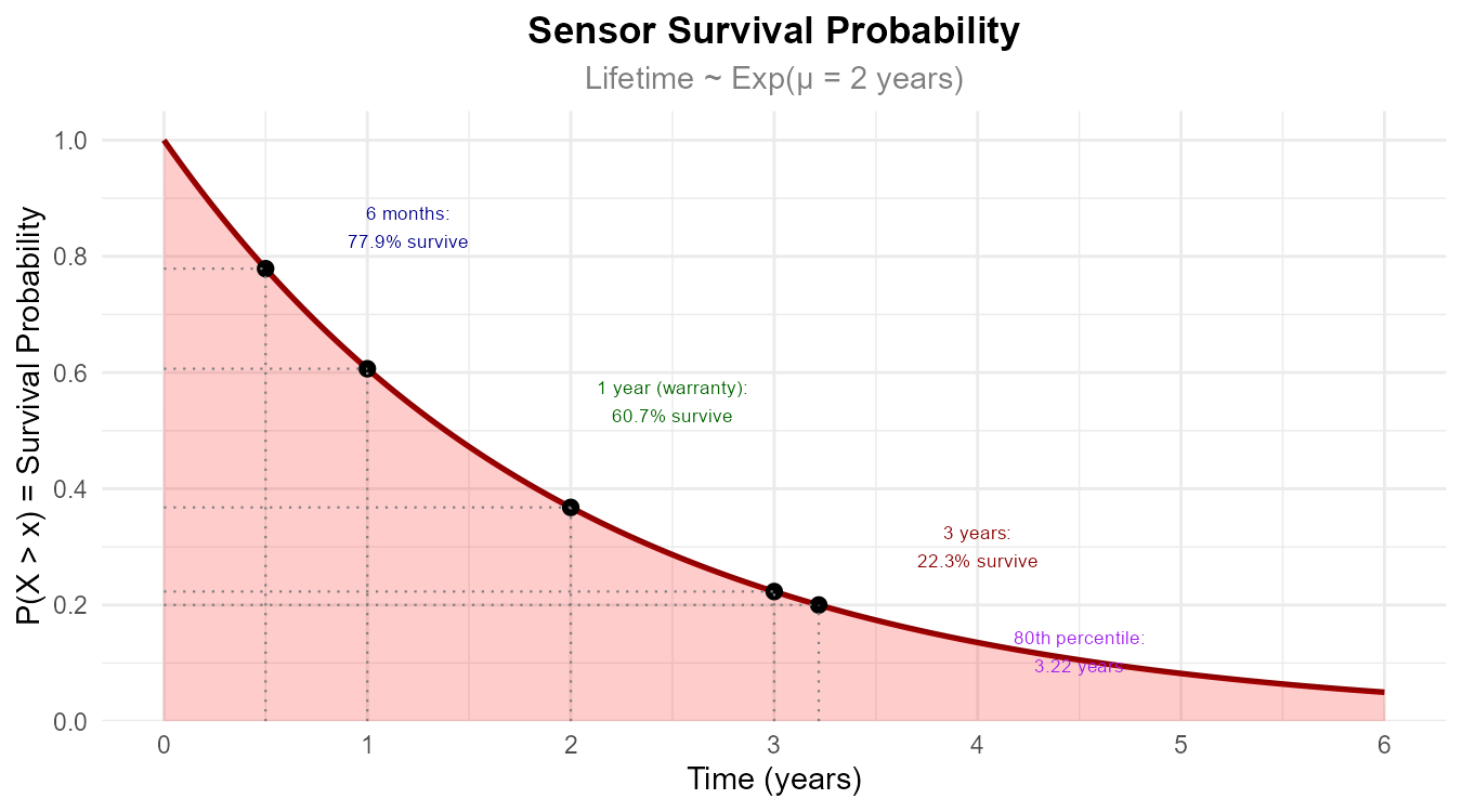
Fig. 6.58 Survival probability decreases exponentially; marked points show key probabilities.

---

6.6.9. Additional Practice Problems

True/False Questions (1 point each)

1. For an exponential distribution, the mean equals the standard deviation.

   Ⓣ or Ⓕ

2. The exponential distribution has support \((-\infty, \infty)\).

   Ⓣ or Ⓕ

3. If \(X \sim \text{Exp}(\lambda = 2)\), then \(E[X] = 2\).

   Ⓣ or Ⓕ

4. The memoryless property states \(P(X > s + t \mid X > s) = P(X > t)\).

   Ⓣ or Ⓕ

5. For \(X \sim \text{Exp}(\lambda)\), \(P(X > x) = e^{-\lambda x}\) for \(x \geq 0\).

   Ⓣ or Ⓕ

6. The median of an exponential distribution is always greater than its mean.

   Ⓣ or Ⓕ

7. If events follow a Poisson process with rate \(\lambda\), the time between events follows \(\text{Exp}(\lambda)\).

   Ⓣ or Ⓕ

8. The exponential PDF achieves its maximum value at \(x = \frac{1}{\lambda}\).

   Ⓣ or Ⓕ

Multiple Choice Questions (2 points each)

9. For \(X \sim \text{Exp}(\lambda = 0.25)\), what is \(E[X]\)?

   Ⓐ 0.25

   Ⓑ 0.5

   Ⓒ 4

   Ⓓ 16

10. For \(X \sim \text{Exp}(\lambda = 0.5)\), what is \(P(X > 2)\)?

    Ⓐ \(e^{-1}\)

    Ⓑ \(e^{-0.5}\)

    Ⓒ \(1 - e^{-1}\)

    Ⓓ \(1 - e^{-0.5}\)

11. For an exponential distribution with mean \(\mu = 5\), what is the rate parameter \(\lambda\)?

    Ⓐ 5

    Ⓑ 0.5

    Ⓒ 0.2

    Ⓓ 25

12. The median of \(\text{Exp}(\lambda)\) is:

    Ⓐ \(\frac{1}{\lambda}\)

    Ⓑ \(\frac{\ln(2)}{\lambda}\)

    Ⓒ \(\frac{2}{\lambda}\)

    Ⓓ \(\lambda\)

13. For \(X \sim \text{Exp}(\lambda = 1)\), what is \(P(X \leq 1)\)?

    Ⓐ \(e^{-1} \approx 0.368\)

    Ⓑ \(1 - e^{-1} \approx 0.632\)

    Ⓒ 0.5

    Ⓓ 1

14. Which distribution would model the number of arrivals in a time period (not the time between arrivals)?

    Ⓐ Exponential

    Ⓑ Normal

    Ⓒ Poisson

    Ⓓ Uniform

Answers to Practice Problems

True/False Answers:

1. True — For \(X \sim \text{Exp}(\lambda)\), both \(E[X] = \frac{1}{\lambda}\) and \(\sigma_X = \frac{1}{\lambda}\). This equality is unique to the exponential distribution.

2. False — The support is \([0, \infty)\). Waiting times cannot be negative.

3. False — \(E[X] = \frac{1}{\lambda} = \frac{1}{2} = 0.5\), not 2.

4. True — This is the definition of the memoryless property.

5. True — This is the survival function, which equals \(1 - F_X(x) = 1 - (1 - e^{-\lambda x}) = e^{-\lambda x}\).

6. False — The median \(\frac{\ln(2)}{\lambda} \approx \frac{0.693}{\lambda}\) is less than the mean \(\frac{1}{\lambda}\) because exponential distributions are right-skewed.

7. True — This is the fundamental connection between Poisson and exponential distributions.

8. False — The PDF achieves its maximum at \(x = 0\), where \(f_X(0) = \lambda\).

Multiple Choice Answers:

9. Ⓒ — \(E[X] = \frac{1}{\lambda} = \frac{1}{0.25} = 4\).

10. Ⓐ — \(P(X > 2) = e^{-0.5 \times 2} = e^{-1}\).

11. Ⓒ — \(\lambda = \frac{1}{\mu} = \frac{1}{5} = 0.2\).

12. Ⓑ — Solving \(e^{-\lambda x_{0.5}} = 0.5\) gives \(x_{0.5} = \frac{\ln(2)}{\lambda}\).

13. Ⓑ — \(P(X \leq 1) = 1 - e^{-1 \times 1} = 1 - e^{-1} \approx 0.632\).

14. Ⓒ — Poisson models counts of events; exponential models time between events.