Slides 📊

3.3. Measures of Variability - Range, Variance, and Standard Deviation

When describing a dataset, knowing where the center lies tells only half the story. Two datasets might share the same mean or median but look entirely different when plotted. This may be because they differ in how widely the values are dispersed. Measures of spread help us quantify this dispersion, providing a more complete picture of our data’s characteristics.

Road Map 🧭

Calculate and interpret the range as a simple spread measure.
Develop the concept of deviations from the mean.
Define and compute the variance and standard deviation.

3.3.1. The Need for Measures of Variability

When using only measures of central tendency, we often lose important information about the data’s distribution. For example:

Two countries might have the same mean family income, but one could have both greater wealth and greater poverty than the other.
Two classes might have the same average test score, but one might have consistent performance while the other has extreme high and low scores.
Two manufacturing processes might produce parts with the same average size, but one might have much tighter tolerances than the other.

Consider the visualization below, which shows two distributions with identical means but different spreads:

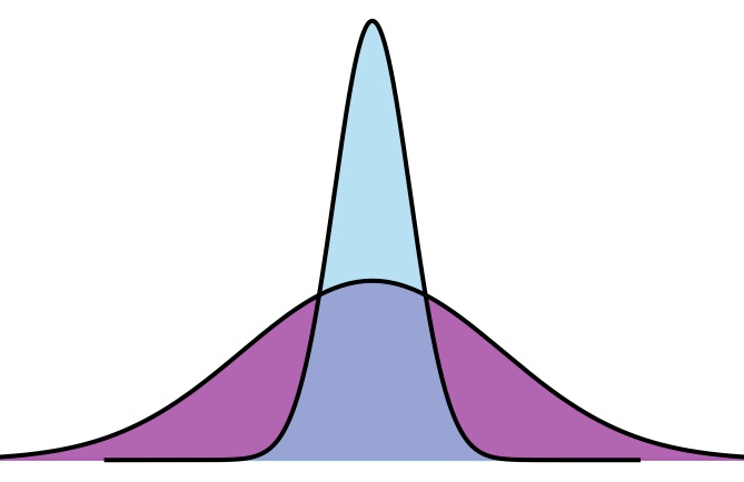
Two distributions with same mean but different spreads — Fig. 3.3 Two distributions with the same mean but different spreads

To fully characterize these distributions, we need measures that quantify the dispersion of values around the center.

3.3.2. Sample Range: The Simplest Measure

The sample range is the most basic measure of spread—simply the difference between the maximum and minimum values in a dataset:

\[\text{Range} = \text{Maximum} - \text{Minimum}\]

Example 💡: Continuing with the pet counts data

We continue to use the pet counts data from Part 1 of Section 3.2.4:

\[\{4, 8, 7, 9, 4, 3, 5, 1, 4\}.\]

The range is \(9 - 1 = 8\).

# Creating the dataset
num_pets <- c(4, 8, 7, 9, 4, 3, 5, 1, 4)

range_pets <- max(num_pets) - min(num_pets)
range_pets  # Returns 8

Limitations of Sample Range

While the range is easy to calculate and understand, it has significant limitations:

It depends only on the two most extreme values, ignoring all other observations.
It is highly sensitive to outliers.
Two very different distributions can have identical ranges.

To illustrate this limitation, consider three different data sets that all have the same range and central tendencies:

Table 3.1 Data sets with the same range and mean but different distributions
Set 1	-15	-1	-0.5	0.5	1	15
Set 2	-15	-3	-1	1	3	15
Set 3	-15	-10	-5	5	10	15

Three datasets with same range but different distributions

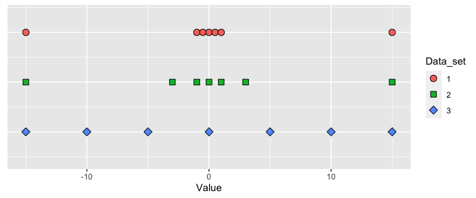
All three datasets have a range of 30 (from -15 to 15) and a mean of 0, but their distributions are clearly different. Set 1 has most values concentrated near the center with only a few extreme points, Set 2 is less concentrated, and Set 3 has values more evenly distributed across the range.

This example demonstrates why we need measures that consider the dispersion of all values in the dataset, not just the extremes.

3.3.3. Sample Variance and Sample Standard Deviation

Deviations from the Mean

To better measure the spread, we need to consider how far each data point lies from a central value, typically the mean. This distance is called a deviation.

For each observation \(x_i\), its deviation from the sample mean is defined as:

\[d_i = x_i - \bar{x}\]

Deviations in Pet Counts Data

Let’s calculate the deviations for our pet counts data set using \(\bar{x} = 5\). The values are recorded in Table 3.2.

Table 3.2 Deviations and Squared Deviations from the Sample Mean
Object	Pet Counts Data	Deviation	Squared deviation
Formula	\(x_i\)	\(x_i - \bar{x}\)	\((x_i - \bar{x})^2\)
Value	\(1\)	\(1-5=-4\)	\((1-5)^2=16\)
	\(3\)	\(3-5=-2\)	\((3-5)^2=4\)
	\(4\)	\(4-5=-1\)	\((4-5)^2=1\)
	\(4\)	\(4-5=-1\)	\((4-5)^2=1\)
	\(4\)	\(4-5=-1\)	\((4-5)^2=1\)
	\(5\)	\(5-5=0\)	\((5-5)^2=0\)
	\(7\)	\(7-5=2\)	\((7-5)^2=4\)
	\(8\)	\(8-5=3\)	\((8-5)^2=9\)
	\(9\)	\(9-5=4\)	\((9-5)^2=16\)
Sum	\(\sum_{i=1}^n x_i = n\bar{x} = 45\)	\(\sum_{i=1}^n (x_i -\bar{x})=\) \(\sum_{i=1}^n x_i -n\bar{x} = 0\)	\(\sum_{i=1}^n (x_i -\bar{x})^2=52\)

From the final row of Table 3.2, we note an important property of deviations; they always sum to zero. This makes it impossible for their average to serve as a meaningful summary for a data set. Instead, we use the squared deviations so that only the magnitudes influence the summary, not their signs. See the right most column of Table 3.2 for the squared deviations of the pet counts data.

If signs are an issue, why not take absolute values?

Indeed, variability metrics which use absolute deviations exist. However, those that use squared deviations are far more widely adopted because of their powerful theoretical properties. We will explore these properties throughout the semester.

Sample Variance, \(s^2\)

We compute the sample variance, denoted by \(s^2\), by taking the sum of all squared deviations, then dividing it by \(n-1\):

\[s^2 = \frac{1}{n-1}\sum_{i=1}^{n}(x_i-\bar{x})^2\]

The sample variance represents the average squared deviation from the mean, although we divide by \(n-1\) rather than \(n\). While the full theoretical explanation is not covered yet, this adjustment is made to correct for bias in the estimation.

Example 💡: Computing the Sample Variance

Let’s calculate the variance for the pet counts example. Most hard work has already been done in Table 3.2. We take the sum of the final column, then divide by \(n-1\).

\[s^2 = \frac{1}{n-1}\sum_{i=1}^{n}(x_i-\bar{x})^2 = \frac{52}{9-1} = 6.5\]

Using R,

num_pets <- c(4, 8, 7, 9, 4, 3, 5, 1, 4)
var(num_pets)  # Returns 6.5

Sample Standard Deviation, \(s\)

While the sample variance is mathematically useful, it has a practical drawback–it’s expressed in the squared scale of the original unit, making interpretations difficult.

We return to the original unit by taking the positive square root of the sample variance. This value is called the sample standard deviation:

\[s = \sqrt{s^2} = \sqrt{\frac{1}{n-1}\sum_{i=1}^{n}(x_i-\bar{x})^2}.\]

Example 💡: Computing the Sample Standard Deviation

For the pet counts example,

\[s = \sqrt{6.5} \approx 2.55.\]

On average, the pet count deviates from the mean by about 2.55 pets.

num_pets <- c(4, 8, 7, 9, 4, 3, 5, 1, 4)
sd(num_pets)  # Returns 2.55

Properties of Variance and Standard Deviation

They are always non-negative.
They equal zero only when all data values are identical.
They increase as the spread of the data increases.
The two measures always increase and decrease together.

3.3.4. Revisiting the Three Datasets with a Shared Range

Let’s return to our three datasets:

Table 3.3 Data sets with the same range and mean but different distributions
Data set	Data values						Variance
1	-15	-1	-0.5	0.5	1	15	75.42
2	-15	-3	-1	1	3	15	78.33
3	-15	-10	-5	5	10	15	116.67

Although all three datasets have the same sample range (30) and sample mean (0), their variances differ substantially. Set 1, with most points concentrated near the center, has the smallest variance. Set 3, with points more spread out, has the largest variance. This illustrates how variance and standard deviation capture differences in distribution that the range misses.

3.3.5. Impact of extreme values

Let us compute the sample range, variance, and standard deviation for the updated pet counts data from Part 2 of Section 3.2.4.

New pet counts data
1	3	4	4	4	5	7	8	9 → 19

Sample range

\[19 - 1 = 18.\]

Sample variance and sample standard deviation

In Part 2 of Section 3.2.4, we computed the new sample mean as \(\bar{x}=6.11\). We must re-compute the squared deviations for all data points using this new value:

Table 3.4 Deviations and Squared Deviations from the Sample Mean
Object	Updated Pet Counts Data	Updated Squared deviation
Formula	\(x_i\)	\((x_i - \bar{x})^2\)
Value	\(1\)	\((1-6.11)^2=26.12\)
	\(3\)	\((3-6.11)^2=9.68\)
	\(4\)	\((4-6.11)^2=4.46\)
	\(4\)	\((4-6.11)^2=4.46\)
	\(4\)	\((4-6.11)^2=4.46\)
	\(5\)	\((5-6.11)^2=1.23\)
	\(7\)	\((7-6.11)^2=0.79\)
	\(8\)	\((8-6.11)^2=3.57\)
	\(19\)	\((9-6.11)^2=166.12\)
Sum	\(\sum_{i=1}^n x_i = n\bar{x} = 55\)	\(\sum_{i=1}^n (x_i -\bar{x})^2=220.8889\)

Then the sample variance is

\[s^2 = \frac{1}{n-1}\sum_{i=1}^n (x_i-\bar{x})^2 = \frac{220.8889}{9} = 27.6111,\]

and the sample standard deviation is

\[s = \sqrt{s^2} = \sqrt{27.6111} = 5.2546.\]

How did the measures of spread change?
Measure	Before update	→	After update
Sample range	8	→	18
Sample variance	6.5	→	27.6111
Sample standard deviation	2.55	→	5.2546

All three measures increased after an extreme value of 19 was added to the data set. Between the sample range and sample standard deviation—both on the data’s original scale—the impact was weaker on the standard deviation. This is because the standard deviation incorporates all data points in its calculation, whereas the sample range depends only on the extremes. The increase in the sample variance is the most dramatic, but this is because it is computed on the squared scale.

3.3.6. Bringing It All Together

Key Takeaways 📝

Central tendency measures alone don’t fully describe a dataset; we also need measures of spread.
The range (max - min) is the simplest spread measure but depends only on the extreme values, which often have the least representative power of the data.
Deviations from the mean always sum to zero. Therefore, we construct a measure of spread with squared deviations.
The sample variance (\(s^2\)) is the average squared deviation from the mean.
The sample standard deviation (\(s\)) is the square root of the sample variance, returning to the original units of measurement.
The three measures are sensitive to extreme values.

3.3.7. Exercises

These exercises build your skills in calculating and interpreting measures of variability: range, variance, and standard deviation.

Exercise 1: Calculating Measures of Variability

A mechanical engineer measures the diameter (in mm) of 8 ball bearings from a production run:

\[\{10.02, 9.98, 10.01, 9.99, 10.03, 9.97, 10.00, 10.00\}\]

Calculate the sample mean (\(\bar{x}\)).
Calculate the sample range.
Complete the following table to find the deviations and squared deviations:

\(x_i\)

\(x_i - \bar{x}\)

\((x_i - \bar{x})^2\)

10.02

9.98

…

…

…
Verify that \(\sum_{i=1}^{n}(x_i - \bar{x}) = 0\).
Calculate the sample variance (\(s^2\)).
Calculate the sample standard deviation (\(s\)).
Interpret the standard deviation in context: “On average, the diameter of a ball bearing deviates from the mean by approximately ___ mm.”

Solution

Part (a): Sample Mean

\[\bar{x} = \frac{10.02 + 9.98 + 10.01 + 9.99 + 10.03 + 9.97 + 10.00 + 10.00}{8} = \frac{80.00}{8} = 10.00 \text{ mm}\]

Part (b): Sample Range

\[\text{Range} = \max - \min = 10.03 - 9.97 = 0.06 \text{ mm}\]

Part (c): Deviations Table

\(x_i\)	\(x_i - \bar{x}\)	\((x_i - \bar{x})^2\)
10.02	0.02	0.0004
9.98	−0.02	0.0004
10.01	0.01	0.0001
9.99	−0.01	0.0001
10.03	0.03	0.0009
9.97	−0.03	0.0009
10.00	0.00	0.0000
10.00	0.00	0.0000
Sum	0.00	0.0028

Part (d): Verify Sum of Deviations

\[\sum_{i=1}^{8}(x_i - \bar{x}) = 0.02 + (-0.02) + 0.01 + (-0.01) + 0.03 + (-0.03) + 0 + 0 = 0 \checkmark\]

This confirms the property that deviations from the mean always sum to zero.

Part (e): Sample Variance

\[s^2 = \frac{1}{n-1}\sum_{i=1}^{n}(x_i - \bar{x})^2 = \frac{0.0028}{8-1} = \frac{0.0028}{7} = 0.0004 \text{ mm}^2\]

Part (f): Sample Standard Deviation

\[s = \sqrt{s^2} = \sqrt{0.0004} = 0.02 \text{ mm}\]

Part (g): Interpretation

“On average, the diameter of a ball bearing deviates from the mean by approximately 0.02 mm.”

This indicates very tight manufacturing tolerances—the bearings are highly consistent.

Exercise 2: Understanding the Limitations of Range

Three different manufacturing processes produce parts with the following measurements (in cm):

Process A: {4.5, 4.9, 5.0, 5.0, 5.1, 5.5}
Process B: {4.5, 4.7, 4.9, 5.1, 5.3, 5.5}
Process C: {4.5, 5.0, 5.0, 5.0, 5.0, 5.5}

Calculate the range for each process.
Calculate the sample mean for each process.
Calculate the sample standard deviation for each process.
Which process produces the most consistent parts? Justify using both range and standard deviation.
Explain why range alone can be misleading when comparing these processes.

Exercise 3: Effect of Outliers on Variability Measures

A data analyst records the response times (in milliseconds) for 10 server requests:

\[\{45, 48, 52, 47, 51, 49, 50, 46, 53, 48\}\]

Calculate the range, variance, and standard deviation.
One request experienced a timeout and took 250 ms. Add this value to the dataset and recalculate all three measures.
Create a table comparing the “before” and “after” values. Calculate the percentage increase for each measure.
Which measure was affected most by the outlier? Which was affected least?
If the analyst wants to report a “typical” level of variability for this server, should they include the timeout value? Justify your answer.

Solution

Part (a): Original Data (n = 10)

Data: {45, 48, 52, 47, 51, 49, 50, 46, 53, 48}

Mean: \(\bar{x} = \frac{489}{10} = 48.9\) ms

Range: \(53 - 45 = 8\) ms

Variance:

\[\sum(x_i - 48.9)^2 = 15.21 + 0.81 + 9.61 + 3.61 + 4.41 + 0.01 + 1.21 + 8.41 + 16.81 + 0.81 = 60.9\]

\[s^2 = \frac{60.9}{9} = 6.7667 \text{ ms}^2\]

Standard Deviation: \(s = \sqrt{6.77} = 2.6013\) ms

Part (b): With Outlier (n = 11)

New data: {45, 48, 52, 47, 51, 49, 50, 46, 53, 48, 250}

New mean: \(\bar{x} = \frac{739}{11} = 67.1818\) ms

Range: \(250 - 45 = 205\) ms

Variance:

The outlier contributes \((250 - 67.1818)^2 = 33,422.49\) to the sum of squared deviations.

\[s^2 = \frac{\sum(x_i - 67.1818)^2}{10} = \frac{36,825.64}{10} = 3,682.5636\text{ ms}^2\]

Standard Deviation: \(s = \sqrt{3721.87} = 60.6841\) ms

Part (c): Comparison Table

Measure	Before	After	% Increase
Range	8 ms	205 ms	2,462%
Variance	6.7667 ms²	3,682.5636 ms²	54322.12%
Std Dev	2.6013 ms	60.6841 ms	2,232.855%

Part (d): Impact Analysis

Most affected: Variance (increased by over 54,000%) — this is because variance uses squared deviations, so the outlier’s effect is amplified
Least affected (on original scale): Standard deviation (2,232%) — still enormous, but less than range
Range increased by 2,462%, similar to standard deviation in percentage terms

All three measures are highly sensitive to outliers. The variance appears most affected because it’s on a squared scale.

Part (e): Should the Outlier Be Included?

It depends on the purpose of the analysis:

If reporting typical server performance:

Exclude the timeout value
Report \(s = 2.60\) ms as the typical variability
Note that timeouts occur occasionally but are exceptional

If assessing overall system reliability:

Include the timeout value
Report that variability is high (\(s = 60.68\) ms) when timeouts occur
This represents the actual user experience

Best practice:

Report both: “Typical response variability is 2.6 ms, but occasional timeouts (approximately 10% of requests) increase overall variability to 61 ms”
Investigate the cause of the timeout separately

Exercise 4: Why Divide by n−1?

This exercise explores the reasoning behind using \(n-1\) in the sample variance formula.

Consider a small population with values: {2, 4, 6}

Calculate the population variance using the formula \(\sigma^2 = \frac{1}{N}\sum_{i=1}^{N}(x_i - \mu)^2\) where \(N = 3\).
List all possible samples of size \(n = 2\) that can be drawn from this population (with replacement). There are 9 such samples.
For each sample, calculate \(s^2\) using \(n-1 = 1\) in the denominator.
Calculate the average of all your \(s^2\) values from part (c).
How does this average compare to the population variance from part (a)? What does this suggest about why we use \(n-1\)?

Solution

Part (a): Population Variance

Population: {2, 4, 6}, \(N = 3\)

Population mean: \(\mu = \frac{2 + 4 + 6}{3} = 4\)

\[\sigma^2 = \frac{(2-4)^2 + (4-4)^2 + (6-4)^2}{3} = \frac{4 + 0 + 4}{3} = \frac{8}{3} = 2.67\]

Part (b): All Samples of Size 2 (with replacement)

Sample	Values
1	{2, 2}
2	{2, 4}
3	{2, 6}
4	{4, 2}
5	{4, 4}
6	{4, 6}
7	{6, 2}
8	{6, 4}
9	{6, 6}

Part (c): Sample Variance for Each Sample

For each sample, \(s^2 = \frac{\sum(x_i - \bar{x})^2}{n-1} = \frac{\sum(x_i - \bar{x})^2}{1}\)

Sample	Values	\(\bar{x}\)	\(s^2\)
1	{2, 2}	2	\(\frac{0+0}{1} = 0\)
2	{2, 4}	3	\(\frac{1+1}{1} = 2\)
3	{2, 6}	4	\(\frac{4+4}{1} = 8\)
4	{4, 2}	3	\(\frac{1+1}{1} = 2\)
5	{4, 4}	4	\(\frac{0+0}{1} = 0\)
6	{4, 6}	5	\(\frac{1+1}{1} = 2\)
7	{6, 2}	4	\(\frac{4+4}{1} = 8\)
8	{6, 4}	5	\(\frac{1+1}{1} = 2\)
9	{6, 6}	6	\(\frac{0+0}{1} = 0\)

Part (d): Average of Sample Variances

\[\text{Average } s^2 = \frac{0 + 2 + 8 + 2 + 0 + 2 + 8 + 2 + 0}{9} = \frac{24}{9} = 2.67\]

Part (e): Comparison and Conclusion

The average of the sample variances (2.67) equals the population variance (2.67) exactly!

This demonstrates why we divide by \(n-1\) instead of \(n\):

When we use \(n-1\), the sample variance \(s^2\) is an unbiased estimator of the population variance \(\sigma^2\)
“Unbiased” means that on average (across all possible samples), \(s^2\) equals \(\sigma^2\)
If we divided by \(n\) instead, the sample variance would systematically underestimate the true population variance
The \(n-1\) correction accounts for the fact that we’re estimating the mean from the same sample we use to calculate variance, which causes us to lose one “degree of freedom”

Exercise 5: Comparing Variability Across Groups

A quality control manager compares two suppliers of electronic components. The failure times (in hours) for samples from each supplier are:

Supplier A (n = 6): {980, 1020, 995, 1010, 1005, 990}
Supplier B (n = 6): {850, 1150, 920, 1080, 970, 1030}

Calculate the mean failure time for each supplier.
Calculate the standard deviation for each supplier.
Which supplier provides more consistent (reliable) components?
The manager wants components with a mean failure time of at least 1000 hours. Which supplier better meets this requirement, considering both the average and consistency?
Calculate the coefficient of variation (CV) for each supplier, defined as \(CV = \frac{s}{\bar{x}} \times 100\%\). What advantage does CV have over standard deviation for comparison?

Exercise 6: Conceptual Understanding

Answer the following conceptual questions about measures of variability.

Can the standard deviation ever be negative? Can it ever be zero? Explain the conditions for each.
If every value in a dataset is increased by 10, what happens to the range, variance, and standard deviation?
If every value in a dataset is multiplied by 3, what happens to the range, variance, and standard deviation?
A dataset has \(\bar{x} = 50\) and \(s = 10\). If a new value of 50 is added to the dataset, will the standard deviation increase, decrease, or stay the same? Explain.
Two datasets have the same mean. Dataset X has a larger range than Dataset Y. Is it possible for Dataset Y to have a larger standard deviation? Explain with an example.
Why do we square the deviations when calculating variance, rather than using absolute values?

Solution

Part (a): Can Standard Deviation Be Negative or Zero?

Negative: No, standard deviation cannot be negative.

It’s defined as the square root of variance
Variance is a sum of squared terms, which are always non-negative
The square root of a non-negative number is non-negative

Zero: Yes, standard deviation can be zero, but only when all values in the dataset are identical.

If all \(x_i = c\) (some constant), then \(\bar{x} = c\)
Every deviation \((x_i - \bar{x}) = 0\)
Sum of squared deviations = 0
\(s = 0\)

Part (b): Adding a Constant to All Values

If every value increases by 10:

Range: Unchanged (both max and min increase by 10, so their difference stays the same)
Variance: Unchanged (deviations from the mean don’t change because the mean also increases by 10)
Standard deviation: Unchanged

Adding a constant shifts all values but doesn’t change their spread.

Part (c): Multiplying All Values by a Constant

If every value is multiplied by 3:

Range: Multiplied by 3 (new range = 3 × old range)
Standard deviation: Multiplied by 3 (new \(s\) = 3 × old \(s\))
Variance: Multiplied by \(3^2 = 9\) (new \(s^2\) = 9 × old \(s^2\))

Multiplying by a constant scales the spread proportionally (or by the square for variance).

Part (d): Adding a Value Equal to the Mean

If we add a value equal to the mean (50), the standard deviation will decrease.

Reasoning:

The new value has deviation = 0 (it’s exactly at the mean)
It adds 0 to the sum of squared deviations
But it increases \(n\) (and thus \(n-1\) in the denominator)
More observations with the same sum of squared deviations → smaller variance → smaller s

Intuitively: adding a value at the center “concentrates” the distribution slightly.

Part (e): Larger Range but Smaller Standard Deviation?

Yes, this is possible.

Example:

Dataset X: {0, 5, 5, 5, 5, 10} — Range = 10, most values at center
Dataset Y: {0, 2, 4, 6, 8, 10} — Range = 10, values spread evenly

Wait, let me recalculate to match the question (X has larger range than Y):

Dataset X: {0, 50, 50, 50, 50, 100} — Range = 100, concentrated at center
Dataset Y: {25, 30, 40, 60, 70, 75} — Range = 50, more evenly spread

For X: \(\bar{x} = 50\), values cluster at 50, so \(s\) is relatively small For Y: \(\bar{x} = 50\), values spread throughout range, so \(s\) is larger

The key insight: range only considers extremes, while standard deviation considers all values. Extreme values can create a large range while the bulk of data stays concentrated.

Part (f): Why Square Deviations Instead of Absolute Values?

We use squared deviations rather than absolute values because:

Mathematical tractability: Squared functions are differentiable everywhere; absolute value has a “kink” at zero that complicates calculus-based analysis
Theoretical properties: Variance has powerful properties in statistical theory: - \(\text{Var}(aX + b) = a^2 \text{Var}(X)\) - For independent variables: \(\text{Var}(X + Y) = \text{Var}(X) + \text{Var}(Y)\)
Connection to normal distribution: The normal distribution is defined using squared terms, and variance/standard deviation connect directly to it
Least squares estimation: Minimizing squared errors is the foundation of regression analysis
Emphasis on larger deviations: Squaring gives more weight to larger deviations, which may be desirable for detecting outliers

Note: The Mean Absolute Deviation (MAD) uses absolute values and is sometimes preferred for its resistance to outliers, but variance remains standard due to its theoretical advantages.

3.3.8. Additional Practice Problems

True/False Questions (1 point each)

The range uses all observations in its calculation.

Ⓣ or Ⓕ
The sum of all deviations from the mean always equals zero.

Ⓣ or Ⓕ
The sample variance is always larger than the sample standard deviation.

Ⓣ or Ⓕ
If the standard deviation is zero, all values in the dataset must be identical.

Ⓣ or Ⓕ
Multiplying every value in a dataset by 2 will double the variance.

Ⓣ or Ⓕ
The sample variance formula divides by \(n-1\) to correct for bias in estimation.

Ⓣ or Ⓕ

Multiple Choice Questions (2 points each)

For the dataset {10, 20, 30, 40, 50}, the sample variance \(s^2\) is calculated by dividing the sum of squared deviations by:

Ⓐ 4

Ⓑ 5

Ⓒ 25

Ⓓ \(\sqrt{5}\)
Two datasets have the same mean of 100. Dataset A has \(s = 5\) and Dataset B has \(s = 15\). Which statement is correct?

Ⓐ Dataset A has more variability

Ⓑ Dataset B has more variability

Ⓒ Both datasets have the same variability

Ⓓ Cannot determine without knowing the ranges
If every observation in a dataset is increased by 25, the standard deviation will:

Ⓐ Increase by 25

Ⓑ Increase by 625

Ⓒ Stay the same

Ⓓ Decrease by 25
A quality engineer compares two processes. Process X has Range = 10 and \(s = 2\). Process Y has Range = 8 and \(s = 3\). Which process is more consistent?

Ⓐ Process X (smaller standard deviation indicates more consistency)

Ⓑ Process Y (smaller range indicates more consistency)

Ⓒ Both are equally consistent

Ⓓ Cannot determine without the means