Slides 📊
11.3. Independent Two-Sample Analysis - Pooled Variance Estimator
The theoretical framework developed in Chapter 11.2 illustrates the foundational ideas of two-sample inference but relies on known population variances. This section addresses the more practical case in which these variances must be estimated from sample data. We continue, however, under the simplifying assumption that the population variances are equal.
Road Map 🧭
Understand the meaning of the equal variance assumption and the concept of pooled variance estimation.
Learn the structure of the pooled variance estimator and use it to estimate the standard error of \(\bar{X}_A - \bar{X}_B\).
Identify the pivotal quantity consistent with the equal variance assumption, and construct hypothesis tests and confidence regions based on their distributional properties.
11.3.1. The Equal Variance Assumption
As we relax the assumption of known population variances, we first consider the constrained cases where:
This assumption states that the populations have the same underlying variability. While the true variance \(\sigma^2\) still remains unknown, the assumption reduces the number of unknown elements in the framework, making the problem slightly simpler.
Meanwhile, the fundamental assumptions introduced in Chapter 11.2.1 must continue to hold throughout the subsequent discussion.
Mathematical Simplification of the Standard Error
In general, the standard error of the point estimator \(\bar{X}_A - \bar{X}_B\) is:
By replacing both \(\sigma^2_A\) and \(\sigma^2_B\) with \(\sigma^2\), the standard error simplifies to:
leaving only one unknown quantity \(\sigma\) to be estimated.
11.3.2. The Pooled Variance Estimator
When both sample variances \(S^2_A\) and \(S^2_B\) estimate the same underlying parameter \(\sigma^2\), we must systematically combine the information from both samples to create a single estimator of the common variance. When samples from two or more populations are used to estimate a single variance, we call the result a pooled variance estimator.
To define a pooled estimator, we cannot simply compute an overall sample variance from the merged dataset. Recall that a sample variance is the average squared distance of data points from a common mean. When we use the combined dataset to compute an overall mean, this does not provide a good estimate of either population mean—especially when our goal is to determine whether the true means differ. Consequently, the overall sample variance also inaccurately represents the true \(\sigma^2\).
Instead, we take the weighted average of the two separate variance estimators \(S_A^2\) and \(S_B^2.\) The pooled variance estimator \(S_p^2\) is defined as:
Understanding the Weights
The weights \((n_A - 1)\) and \((n_B - 1)\) in Equation (11.1) represent the degrees of freedom associated with the individual sample variances. These weights ensure that the contribution of each sample is proportional to the relative sample size. As \(n_A\) grows larger relative to \(n_B\), for example, \(S_p^2\) moves closer to the sample variance of Sample A.
The Pooled Estimator is Still an Average of Squared Distances
Note that each additive term in the numerator can be rewritten as the sum of squared distances between data points and their appropriate sample mean. For Sample A:
A similar result holds for Sample B. Using this, \(S^2_p\) can be represented more explicitly as:
Equation (11.2) makes it clear that \(S^2_p\) is still an average of squared deviations from a mean. The only change is that certain data points deviate from Mean A, while the rest deviate from Mean B.
Why Divide by \(n_A + n_B -2\)?
(a) Number of “free” data points
Degrees of freedom is a measure of how many “free” data points there are in a dataset. It usually coincides with the total number of observations subtracted by the number of other parameters estimated to construct the estimator of focus. We have \(n_A + n_B\) total observations, and two parameters—\(\mu_A\) and \(\mu_B\)—were replaced with their estimators \(\bar{X}_A\) and \(\bar{X}_B\) to construct \(S^2_p\).
(b) Correct Normalization for the Weights
For \(S^2_p\) to serve as a weighted average, the denominator must be the sum of all weights used in the numerator. \((n_A - 1) + (n_B - 1) = n_A + n_B - 2\).
(c) Makes \(S^2_p\) Unbiased
\(S^2_p\) as defined above is an unbiased estimator for the common variance \(\sigma^2\) when the equal variance assumption holds.
\[\begin{split}E[S^2_p] &= E\left[\frac{(n_A - 1)S^2_A + (n_B - 1)S^2_B}{n_A + n_B - 2}\right]\\ &= \frac{(n_A - 1)E[S^2_A] + (n_B - 1)E[S^2_B]}{n_A + n_B - 2}\end{split}\]From single-sample theory, we know that the individual sample variances are unbiased:
\[E[S^2_A] = \sigma^2_A \quad \text{ and } \quad E[S^2_B] = \sigma^2_B.\]In addition, both equal \(\sigma^2\) under the equal variance assumption. This implies:
\[\begin{split}E[S^2_p] &= \frac{(n_A - 1)\sigma^2 + (n_B - 1)\sigma^2}{n_A + n_B - 2}\\ &=\frac{\sigma^2[(n_A - 1) + (n_B - 1)]}{n_A + n_B - 2}\\ &= \frac{\sigma^2(n_A + n_B - 2)}{n_A + n_B - 2} = \sigma^2\end{split}\]Therefore, \(S^2_p\) is unbiased.
11.3.3. Estimated Standard Error with Pooled Variance
Recall the true standard error for the point estimator \(\bar{X}_A - \bar{X}_B\) was:
The estimated standard error \(\widehat{SE}_p\) is obtained by replacing the unknown \(\sigma\) with the pooled standard deviation estimator \(S_p = \sqrt{S^2_p}\):
Example 💡: Is It Better to Balance the Sample Size?
Two researchers are studying a pair of Populations A and B, which are assumed to have the same true variance. Researcher 1 designs the experiment with \(n_A = n_B = 10\), while Researcher 2 uses \(n_A = 15, n_B = 5\).
Q1. How do the degrees of freedom compare between the two designs?
In both cases, \(df=n_A + n_B - 2 = 18\). The degrees of freedom are equal.
Q2. Which design will have a smaller true standard error? Explain why.
The true standard error for Researcher 1 is:
\[\sigma \sqrt{\frac{1}{10} + \frac{1}{10}} \approx 0.4472 \sigma .\]For Researcher 2,
\[\sigma \sqrt{\frac{1}{15} + \frac{1}{5}} \approx 0.5164 \sigma .\]The standard error for Researcher 2 is approximately 15% larger than the standard error for Researcher 1. In general, when the total sample size is fixed and the population variances are equal, the smallest possible standard error is achieved with balanced sample sizes.
Q3. In what scenarios might one design be favored over the other?
The design by Researcher 2 would be chosen if it is much more costly to sample from one population than the other, or if the samples are already imbalanced and there are no resources to collect additional data.
If there are no serious difference in sampling costs between the two populations, we would always prefer to have balanced samples, since this leads to a more precise inference without changing the overall cost significantly.
11.3.4. Hypothesis Testing for Independent Two Samples with Equal Variance Assumption
In the four-step framework of hypothesis testing, Steps 1, 2, and 4 are identical to the case with known population variances (see Chapter 11.2 to review the details). We focus our discussion on Step 3, where the key change occurs.
The t-Test Statistic
Recall the common structure of all previously learned test statistics:
Our new test statistic will follow the same format. The estimator is \(\bar{X}_A - \bar{X}_B\), the null value \(\Delta_0\), and the standard error \(\sigma\sqrt{\frac{1}{n_A} + \frac{1}{n_B}}\). Since we do not know the value of \(\sigma\), however, we must replace it with its estimator, \(S_p\). By putting the components together, we get:
When
all assumptions introduced in Chapter 11.2.1 hold,
the true variances are indeed equal, and
the null hypothesis is true,
the test statistic follows a \(t\)-distribution with \(df = n_A + n_B - 2\). The additional uncertainty from estimating \(\sigma^2\) with \(S^2_p\) manifests as the heavier tails characteristic of \(t\)-distributions.
The \(p\)-Values
The \(p\)-value computation reflects the new distribution of the \(t\)-test statistic. Denoting the observed \(t\)-test statistic as \(t_{TS}\), the \(p\)-values for the three hypothesis types are summarized in the table below.
\(p\)-values for independent two-sample tests (unknown pooled variance) |
|
|---|---|
Upper-tailed |
\[P(T_{n_A + n_B -2} > t_{TS})\]
df <- nA + nB - 2
pt(t_ts, df=df, lower.tail=FALSE)
|
Lower-tailed |
\[P(T_{n_A + n_B -2} < t_{TS})\]
df <- nA + nB - 2
pt(t_ts, df=df)
|
Two-tailed |
\[2P(T_{n_A + n_B -2} < -|t_{TS}|) \quad \text{ or } \quad 2P(T_{n_A + n_B -2} > |t_{TS}|)\]
df <- nA + nB - 2
#Two options:
2 * pt(-abs(t_ts), df=df)
2 * pt(abs(t_ts),df=df, lower.tail=FALSE)
|
Example 💡: Dexterity Skill Assessment
A group of 15 new employees participated in a manual dexterity test alongside 20 experienced industrial workers at a high-precision manufacturing company. Skill levels were assessed using test scores from both groups, as shown in the table below:
Group |
\(n\) |
Sample mean |
Sample sd |
|---|---|---|---|
New |
15 |
35.12 |
4.31 |
Senior |
20 |
37.32 |
3.83 |
Perform a hypothesis test to determine if the skill levels for the new employees are lower on average than the senior workers. Use the significance level of \(\alpha=0.05\).
Step 1: Define the parameters
We let \(\mu_{new}\) be the true mean test score of all new employees at this company. Let \(\mu_{exp}\) be the true mean score for the population of experienced employees.
Step 2: Write the Hypotheses
The test can also be defined in terms of \(\mu_{new}-\mu_{exp}\), in which case a lower-tailed test is appropriate. We continue with \(\mu_{exp}-\mu_{new}\) and an upper-tailed test.
The test statistic, degrees of freedom, and p-value
The point estimate of the difference is:
\[\bar{x}_{exp} - \bar{x}_{new} = 37.32 - 35.12 = 2.2\]The pooled variance estimate is:
\[\begin{split}s^2_p &= \frac{(n_{exp} - 1)s^2_{exp} + (n_{new} - 1)s^2_{new}}{n_{exp} + n_{new} - 2}\\ &= \frac{(20 - 1)(3.83)^2 + (15 - 1)(4.31)^2}{20 + 15 - 2} = 16.3265\end{split}\]The estimated standard error is:
\[SE_p = s_p \sqrt{\frac{1}{n_{exp}}+\frac{1}{n_{new}}} = \sqrt{16.3265}\sqrt{\frac{1}{20} + \frac{1}{15}} \approx 1.3801\]Putting together, the observed test statistic is:
\[t_{TS} = \frac{(\bar{x}_{exp} - \bar{x}_{new}) - \Delta_0}{SE_p} = \frac{2.2-0}{1.3801} = 1.5941\]Under the null hypothesis, the random variable \(T_{TS}\) follows a \(t\)-distribution with \(df = 20+15-2=33\). Therefore, the upper-tailed p-value is
\[p = P(T_{33} > 1.5941) = 0.0602\]
Decision and Conclusion
Since \(p = 0.0602 > 0.05\), we fail to reject the null hypothesis. The data does not provide sufficient evidence to support the claim that the mean dexterity test score is higher for experienced workers than for new workers.
11.3.5. Confidence Regions
For confidence interval construction, we use the studentization of \(\bar{X}_A - \bar{X}_B\) as the pivotal quantity:
When all the assumptions hold, \(T\) follows a \(t\)-distribution with \(df = n_A + n_B - 2\). The resulting \(100(1-\alpha)\%\) confidence interval for \(\mu_A - \mu_B\) is:
Again, the confidence interval follows a familiar format:
It is centered at the point estimate \(\bar{x}_A - \bar{x}_B\)
The margin of error (ME) is a product of a critical value and the estimated standard error.
The table below summarizes all three types of confidence regions for the difference in two means, when the pooled estimator is used for the unknown variances:
\(100 \cdot C \%\) Confidence regions for difference in means (unknown pooled variance) |
|
|---|---|
Confidence interval |
\[(\bar{x}_A - \bar{x}_B) \pm t_{\alpha/2, n_A + n_B - 2} \cdot S_p\sqrt{\frac{1}{n_A} + \frac{1}{n_B}}\]
|
Lower confidence bound |
\[(\bar{x}_A - \bar{x}_B) - t_{\alpha, n_A + n_B - 2} \cdot S_p\sqrt{\frac{1}{n_A} + \frac{1}{n_B}}\]
|
Upper confidence bound |
\[(\bar{x}_A - \bar{x}_B) + t_{\alpha, n_A + n_B - 2} \cdot S_p\sqrt{\frac{1}{n_A} + \frac{1}{n_B}}\]
|
The critical values can be computed using the R code:
upper_tail_prob <- alpha #or alpha/2 depending on the type
df <- nA + nB - 2
qt(upper_tail_prob, df=df, lower.tail=FALSE)
Example 💡: Dexterity Skill Assessment, Continued
For the dexterity skill comparison problem, compute the \(95\%\) confidence region that gives an equivalent result to the previously performed hypothesis test. Interpret the result and explain how it is consistent with the test result.
Group |
\(n\) |
Sample mean |
Sample sd |
|---|---|---|---|
New |
15 |
35.12 |
4.31 |
Senior |
20 |
37.32 |
3.83 |
Which confidence region?
Let us continue to use the difference \(\mu_{exp} - \mu_{new}\). The duality of hypothesis tests and confidence regions discussed in Chapter 10.3.1 still hold. When all other experimental settings match, an upper-tailed hypothesis gives a consistent result with a lower confidence bound.
Compute the confidence region
From the previous example, we know:
\(\bar{x}_{exp} - \bar{x}_{new} = 2.2\)
\(\widehat{SE}_p = s_p\sqrt{\frac{1}{n_A} + \frac{1}{n_B}} = \approx 1.3801\)
\(df = 33\)
The critical value \(t_{0.05, 33}\) is:
qt(0.05, df=33, lower.tail=FALSE)
# returns 1.69236
Then finally, the lower confidence bound is:
Interpretation of the Confidence Bound
With \(95\%\) confidence, the true difference in mean test scores (\(\mu_{exp}-\mu_{new}\)) between the two employee groups lies above the lower bound of \(-0.135626\).
Connection to the Hypothesis Test
We were not able to reject the null hypothesis that the true difference was less than or equal to the null value \(\Delta_0 = 0\) at \(\alpha=0.05\). This is consistent with the fact that the null value is inside the plausible region indicated by the \(95\%\) lower confidence bound.
11.3.6. Bringing It All Together
Key Takeaways 📝
Pooled variance procedures assume equal population variances \((\sigma^2_A = \sigma^2_B)\).
The pooled variance estimator \(S^2_p = \frac{(n_A - 1)S^2_A + (n_B - 1)S^2_B}{n_A + n_B - 2}\) combines information from both samples using weights proportional to degrees of freedom.
When the equal variance assumption holds, the random variable \(\frac{(\bar{X}_A - \bar{X}_B)-(\mu_A - \mu_B)}{\widehat{SE}_p}\) follows a \(t\)-distribution with \(df = n_A + n_B - 2\). Both hypothesis testing and confidence regions are constructed using the same core ideas as previously used, but using this new \(t\)-distribution.
11.3.7. Exercises
Exercise 1: Understanding the Equal Variance Assumption
For each scenario, discuss whether the equal variance assumption seems reasonable and justify your answer.
Comparing exam scores between two sections of the same course taught by the same instructor.
Comparing annual salaries between software engineers and marketing managers at a tech company.
Comparing reaction times between participants who drank coffee vs. decaf (same amount of liquid).
Comparing crop yields between two adjacent fields using the same fertilizer and irrigation.
Comparing home prices in a luxury neighborhood vs. a middle-class neighborhood.
Solution
Part (a): Exam scores — REASONABLE ✓
Students in both sections experience similar teaching methods, exam difficulty, and grading standards. Variability in scores should be similar across sections.
Part (b): Salaries — NOT REASONABLE ✗
Software engineers and marketing managers have different pay structures. Engineers may have more variable pay due to bonuses, stock options, and wide skill ranges. Different job functions typically have different variance structures.
Part (c): Reaction times — REASONABLE ✓
The same population of participants is randomly assigned to conditions. Individual variation in baseline reaction time should be similar in both groups. The treatment (caffeine) might affect means but likely not variances dramatically.
Part (d): Crop yields — REASONABLE ✓
Adjacent fields with identical treatment should have similar environmental variability. The same soil quality, weather, and farming practices suggest comparable variance.
Part (e): Home prices — NOT REASONABLE ✗
Luxury homes typically have much higher price variability (range from expensive to extremely expensive) compared to middle-class homes (more uniform pricing). The scales of variability are fundamentally different.
Exercise 2: Computing the Pooled Variance Estimator
Two independent samples yield the following results:
Sample A: \(n_A = 12\), \(s^2_A = 25.6\)
Sample B: \(n_B = 18\), \(s^2_B = 32.4\)
Calculate the pooled variance estimator \(s^2_p\).
Calculate the pooled standard deviation \(s_p\).
Determine the degrees of freedom for the pooled procedure.
If \(\bar{x}_A = 45\) and \(\bar{x}_B = 52\), calculate the estimated standard error \(\widehat{SE}_p\).
Verify that \(s^2_p\) is between \(s^2_A\) and \(s^2_B\).
Solution
Part (a): Pooled variance
Part (b): Pooled standard deviation
Part (c): Degrees of freedom
Part (d): Estimated standard error
Part (e): Verification
Since \(s^2_A = 25.6 < s^2_p = 29.73 < s^2_B = 32.4\), the pooled variance lies between the individual sample variances. ✓
This makes sense because \(s^2_p\) is a weighted average of \(s^2_A\) and \(s^2_B\), with weights proportional to degrees of freedom. Since \(n_B > n_A\), the pooled variance is closer to \(s^2_B\).
R verification:
n_A <- 12; n_B <- 18
s2_A <- 25.6; s2_B <- 32.4

s2_p <- ((n_A - 1) * s2_A + (n_B - 1) * s2_B) / (n_A + n_B - 2)  # 29.73
s_p <- sqrt(s2_p)  # 5.453
df <- n_A + n_B - 2  # 28
SE_p <- s_p * sqrt(1/n_A + 1/n_B)  # 2.033
Exercise 3: Effect of Sample Size on Pooled Variance
Consider two scenarios with the same sample variances but different sample sizes:
Scenario 1: \(n_A = 10\), \(n_B = 10\), \(s^2_A = 20\), \(s^2_B = 40\)
Scenario 2: \(n_A = 50\), \(n_B = 10\), \(s^2_A = 20\), \(s^2_B = 40\)
Calculate \(s^2_p\) for both scenarios.
Calculate the estimated standard error for both scenarios.
Explain why the pooled variances differ despite identical \(s^2_A\) and \(s^2_B\).
Which scenario has a smaller standard error? Why?
Solution
Part (a): Pooled variances
Scenario 1 (\(n_A = n_B = 10\)):
Scenario 2 (\(n_A = 50\), \(n_B = 10\)):
Part (b): Estimated standard errors
Scenario 1:
Scenario 2:
Part (c): Why pooled variances differ
The pooled variance is a weighted average with weights \((n_A - 1)\) and \((n_B - 1)\). In Scenario 1, weights are equal (9 and 9), so \(s^2_p\) is exactly midway between 20 and 40.
In Scenario 2, Sample A has weight 49 while Sample B has weight 9. The pooled variance is pulled strongly toward \(s^2_A = 20\), giving \(s^2_p = 23.10\).
Part (d): Smaller standard error
Scenario 2 has the smaller standard error (1.664 vs. 2.449). Two factors contribute:
Lower pooled variance (23.10 vs. 30)
Larger total sample size (60 vs. 20), which reduces \(\sqrt{1/n_A + 1/n_B}\)
R verification:
# Scenario 1
s2_p_1 <- (9*20 + 9*40)/18  # 30
SE_1 <- sqrt(s2_p_1) * sqrt(1/10 + 1/10)  # 2.449

# Scenario 2
s2_p_2 <- (49*20 + 9*40)/58  # 23.10
SE_2 <- sqrt(s2_p_2) * sqrt(1/50 + 1/10)  # 1.664
Exercise 4: Two-Tailed Pooled t-Test
A quality engineer compares the breaking strength (in Newtons) of two types of plastic connectors. The populations are assumed to have equal variances.
Type A: \(n_A = 15\), \(\bar{x}_A = 245\), \(s_A = 18\)
Type B: \(n_B = 20\), \(\bar{x}_B = 232\), \(s_B = 22\)
Test whether the mean breaking strengths differ at α = 0.05.
Solution
Step 1: Define the parameters
Let \(\mu_A\) = true mean breaking strength (N) for Type A connectors. Let \(\mu_B\) = true mean breaking strength (N) for Type B connectors.
Both population standard deviations are unknown but assumed equal.
Step 2: State the hypotheses
Step 3: Calculate the test statistic and p-value
Pooled variance:
Pooled standard deviation: \(s_p = \sqrt{416.12} = 20.40\)
Estimated standard error:
Test statistic:
Degrees of freedom: \(df = 15 + 20 - 2 = 33\)
P-value (two-tailed):
Step 4: Decision and Conclusion
Since p-value = 0.071 > α = 0.05, fail to reject H₀.
The data does not give support (p-value = 0.071) to the claim that the mean breaking strengths of the two connector types are different. While Type A shows a higher sample mean (245 vs. 232 N), this difference is not statistically significant at the 5% level.
R verification:
n_A <- 15; n_B <- 20
xbar_A <- 245; xbar_B <- 232
s_A <- 18; s_B <- 22

s2_p <- ((n_A-1)*s_A^2 + (n_B-1)*s_B^2) / (n_A + n_B - 2)  # 416.12
s_p <- sqrt(s2_p)  # 20.40
SE_p <- s_p * sqrt(1/n_A + 1/n_B)  # 6.969

t_ts <- (xbar_A - xbar_B) / SE_p  # 1.866
df <- n_A + n_B - 2  # 33
p_value <- 2 * pt(abs(t_ts), df, lower.tail = FALSE)  # 0.0712
Exercise 5: Complete Diagnostic Analysis - Pooled T-Test Assumptions
Before conducting a pooled two-sample t-test, we must verify the assumptions are satisfied. This exercise provides a complete diagnostic analysis workflow.
A manufacturing engineer compares the tensile strength (MPa) of steel samples from two production lines. The goal is to determine if the production lines differ in mean strength.
Sample data summary:
Line A: n_A = 18, x̄_A = 485.2, s_A = 28.5
Line B: n_B = 22, x̄_B = 512.8, s_B = 32.1
Diagnostic Plots:
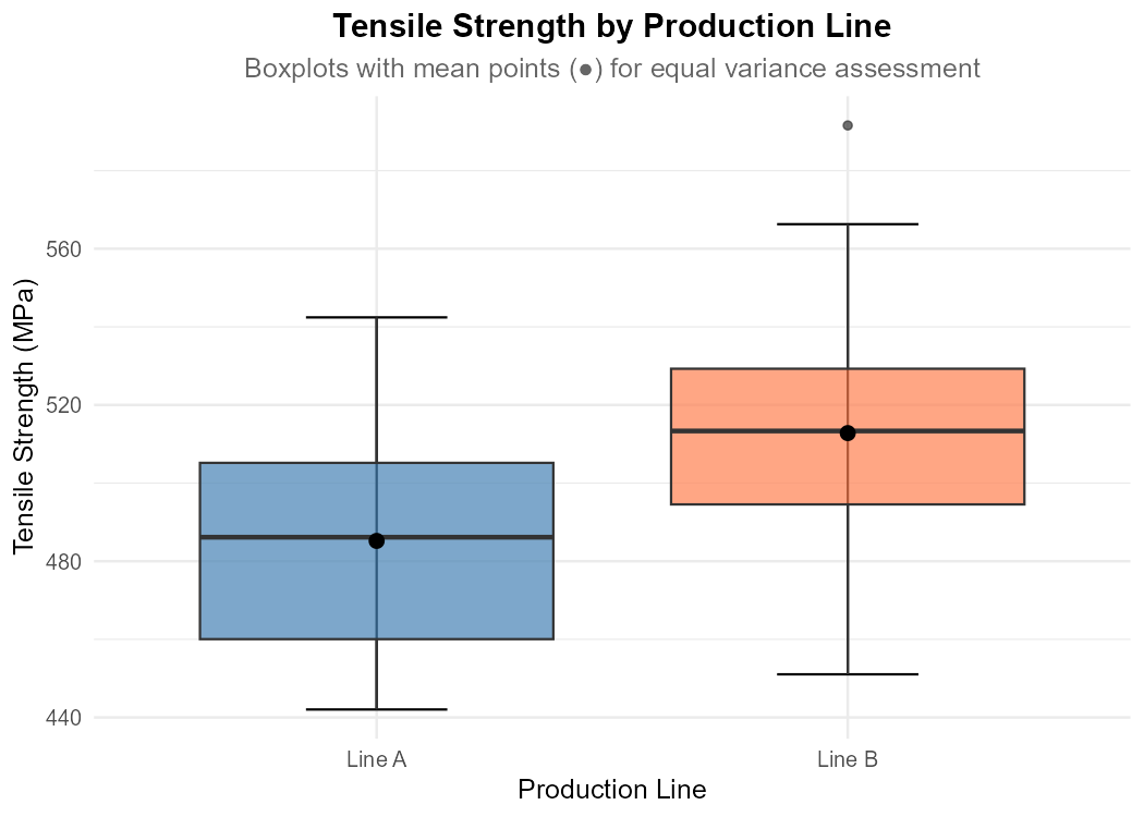
Fig. 11.3 Side-by-side boxplots with mean points (black dots)
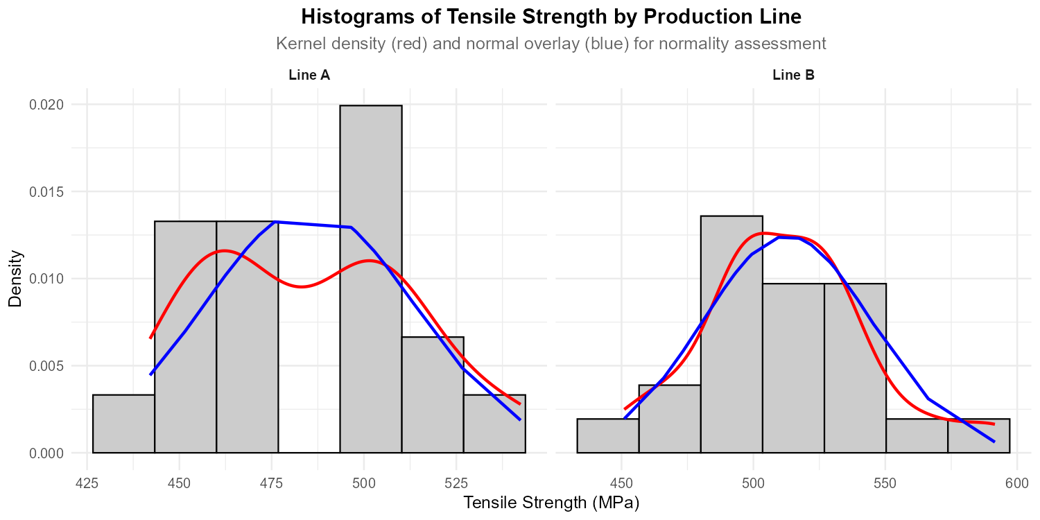
Fig. 11.4 Faceted histograms with kernel density (red) and normal overlay (blue)
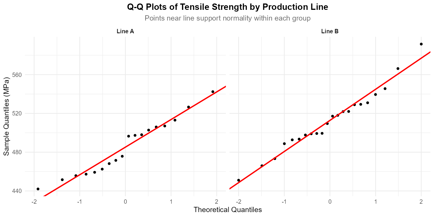
Fig. 11.5 Faceted QQ-plots for each production line
What are the assumptions required for a valid pooled two-sample t-test?
Using the boxplots, visually assess whether the equal variance assumption seems reasonable. What features do you compare?
Calculate the ratio of sample standard deviations. Does it satisfy the rule of thumb (ratio ≤ 2)?
Using the faceted histograms, assess normality within each group. Are there any concerns?
Using the faceted QQ-plots, confirm your normality assessment from part (d).
Based on your diagnostic analysis (parts b-e), should the pooled method be appropriate? Justify your answer.
Conduct the pooled t-test at α = 0.05 using the complete four-step framework.
Solution
Part (a): Assumptions for pooled two-sample t-test
Independence: Samples are independent from each other and within each group
Normality: Both populations are approximately normally distributed (or sample sizes are large enough for CLT)
Equal variances: Both populations have the same variance (σ<sup>2</sup>_A = σ<sup>2</sup>_B)
Part (b): Visual assessment of equal variance
From the boxplots, we compare:
Box lengths (IQR): The boxes for Lines A and B have similar lengths
Whisker lengths: Total spread from whisker to whisker is comparable
Overall spread: Neither group shows dramatically different variability
Visual assessment: The equal variance assumption appears reasonable ✓
Part (c): SD ratio calculation
Since 1.13 ≤ 2, the rule of thumb supports the equal variance assumption ✓
Part (d): Normality assessment from histograms
Line A: The histogram shows an approximately symmetric, unimodal distribution. The kernel density (red) and normal curve (blue) align reasonably well.
Line B: The histogram also appears approximately symmetric and unimodal. Minor random variation is expected with these sample sizes.
Assessment: Both groups show approximate normality ✓
Part (e): Normality assessment from QQ-plots
Line A: Points fall close to the reference line with no systematic curvature. Minor deviations in the tails are within expected random variation.
Line B: Similar pattern—points track the reference line well with acceptable random scatter.
Assessment: QQ-plots confirm approximate normality in both groups ✓
Part (f): Should pooled method be used?
Yes, the pooled method is appropriate because:
✓ Independence is assumed by study design
✓ Normality is supported by histograms and QQ-plots for both groups
✓ Equal variances: SD ratio = 1.13 ≤ 2, and boxplots show similar spreads
All three assumptions for the pooled t-test are reasonably satisfied.
Part (g): Pooled t-test (four-step framework)
Step 1: Define the parameters
Let μ_A = true mean tensile strength (MPa) for Line A Let μ_B = true mean tensile strength (MPa) for Line B
Both population standard deviations are unknown but assumed equal.
Step 2: State the hypotheses
In words: H<sub>0</sub> states the production lines have equal mean tensile strength. Hₐ states the mean tensile strengths differ.
Step 3: Check assumptions and calculate test statistic
Assumption checks:
Independence: Samples are from independent production processes ✓
Equal variances: SD ratio = 32.1/28.5 = 1.13 ≤ 2 ✓
Normality: Histograms and QQ-plots support approximate normality in both groups ✓
Pooled variance:
Estimated standard error:
Test statistic:
Degrees of freedom: df = 18 + 22 - 2 = 38
P-value (two-tailed):
Step 4: Decision and Conclusion
Since p-value = 0.0070 < α = 0.05, reject H<sub>0</sub>.
Conclusion: At the 0.05 significance level, there is sufficient evidence to conclude that the true mean tensile strengths differ between the two production lines (p = 0.007). Line B produces steel with higher mean tensile strength (512.8 vs 485.2 MPa). This difference of 27.6 MPa may have practical significance for product quality specifications.
R verification:
n_A <- 18; n_B <- 22
xbar_A <- 485.2; xbar_B <- 512.8
s_A <- 28.5; s_B <- 32.1

# SD ratio check
max(s_A, s_B) / min(s_A, s_B)  # 1.13 ✓

# Pooled variance
s2_p <- ((n_A-1)*s_A^2 + (n_B-1)*s_B^2) / (n_A + n_B - 2)  # 932.81
s_p <- sqrt(s2_p)  # 30.54
SE_p <- s_p * sqrt(1/n_A + 1/n_B)  # 9.68

# Test statistic and p-value
t_ts <- (xbar_A - xbar_B) / SE_p  # -2.851
df <- n_A + n_B - 2  # 38
p_value <- 2 * pt(t_ts, df)  # 0.0070
Exercise 6: Upper-Tailed Pooled t-Test
A manufacturing company claims that experienced workers (> 2 years) have higher dexterity scores than new workers. The population variances are assumed equal.
Experienced: \(n_{exp} = 20\), \(\bar{x}_{exp} = 37.32\), \(s_{exp} = 3.83\)
New: \(n_{new} = 15\), \(\bar{x}_{new} = 35.12\), \(s_{new} = 4.31\)
Test the company’s claim at α = 0.05.
Solution
Step 1: Define the parameters
Let \(\mu_{exp}\) = true mean dexterity score for experienced workers. Let \(\mu_{new}\) = true mean dexterity score for new workers.
Step 2: State the hypotheses
Testing if experienced workers score higher:
Step 3: Calculate the test statistic and p-value
Pooled variance:
Pooled standard deviation: \(s_p = \sqrt{16.33} = 4.041\)
Estimated standard error:
Test statistic:
Degrees of freedom: \(df = 33\)
P-value (upper-tailed):
Step 4: Decision and Conclusion
Since p-value = 0.060 > α = 0.05, fail to reject H₀.
The data does not give support (p-value = 0.060) to the claim that experienced workers have higher mean dexterity scores than new workers. While the sample difference favors experienced workers (37.32 vs. 35.12), this is not statistically significant at α = 0.05.
R verification:
n_exp <- 20; n_new <- 15
xbar_exp <- 37.32; xbar_new <- 35.12
s_exp <- 3.83; s_new <- 4.31

s2_p <- ((n_exp-1)*s_exp^2 + (n_new-1)*s_new^2) / (n_exp + n_new - 2)
SE_p <- sqrt(s2_p) * sqrt(1/n_exp + 1/n_new)
t_ts <- (xbar_exp - xbar_new) / SE_p  # 1.594
p_value <- pt(t_ts, df = 33, lower.tail = FALSE)  # 0.0602
Exercise 7: Confidence Interval - Pooled Method
A biomedical researcher compares recovery times (days) for two surgical techniques. The equal variance assumption is satisfied.
Technique A: \(n_A = 18\), \(\bar{x}_A = 12.4\), \(s_A = 2.8\)
Technique B: \(n_B = 22\), \(\bar{x}_B = 14.1\), \(s_B = 3.2\)
Construct a 95% confidence interval for \(\mu_A - \mu_B\).
Interpret the confidence interval in context.
Does the interval suggest one technique is better? Explain.
If we want to support the claim that “Technique A is not slower than Technique B,” compute and interpret the appropriate one-sided 95% confidence bound.
Solution
Part (a): 95% Confidence Interval
Pooled variance:
Pooled standard deviation: \(s_p = 3.028\)
Estimated standard error:
Critical value: \(t_{0.025, 38} = 2.024\)
Point estimate: \(\bar{x}_A - \bar{x}_B = 12.4 - 14.1 = -1.7\) days
Margin of error: \(ME = 2.024 \times 0.963 = 1.950\)
95% CI: \(-1.7 \pm 1.950 = (-3.65, 0.25)\) days
Part (b): Interpretation
We are 95% confident that the true difference in mean recovery times (Technique A minus Technique B) is between -3.65 and 0.25 days. Negative values indicate Technique A has shorter recovery times.
Part (c): Does one technique appear better?
The interval contains both negative and positive values, so we cannot definitively conclude one technique is better at the 95% confidence level. However, most of the interval is negative, suggesting Technique A may lead to faster recovery, but more data is needed.
Part (d): 95% Upper Confidence Bound
If our goal is to show “Technique A is not slower than B” (i.e., \(\mu_A - \mu_B \leq 0\)), this corresponds to a lower-tailed alternative \(H_a: \mu_A - \mu_B < 0\). Per the duality rule, a lower-tailed alternative pairs with an upper confidence bound.
For a 95% UCB, use \(t_{0.05, 38} = 1.686\):
We are 95% confident that \(\mu_A - \mu_B \leq -0.08\) days.
Interpretation: Since the UCB is below 0, this supports that Technique A’s mean recovery time is not longer than Technique B’s. In fact, the data suggest A may be slightly faster on average.
Confidence Bound ↔ Hypothesis Test Duality:
Upper-tailed Hₐ (>) → Use LCB → Evidence if LCB > θ₀
Lower-tailed Hₐ (<) → Use UCB → Evidence if UCB < θ₀
R verification:
n_A <- 18; n_B <- 22
xbar_A <- 12.4; xbar_B <- 14.1
s_A <- 2.8; s_B <- 3.2
df <- n_A + n_B - 2  # 38

s2_p <- ((n_A-1)*s_A^2 + (n_B-1)*s_B^2) / df  # 9.166
SE_p <- sqrt(s2_p) * sqrt(1/n_A + 1/n_B)  # 0.962

t_crit_one <- qt(0.05, df, lower.tail = FALSE)  # 1.686
point_est <- xbar_A - xbar_B  # -1.7
UCB <- point_est + t_crit_one * SE_p  # -0.08
Exercise 8: Duality - CI and Hypothesis Test
Using the data from Exercise 6 (Techniques A and B):
Conduct a two-tailed hypothesis test at α = 0.05.
Verify that the test conclusion is consistent with the 95% CI from Exercise 6.
Calculate the p-value and explain what it means.
At what confidence level would the interval just barely exclude zero?
Solution
Part (a): Hypothesis Test
Step 1: Let \(\mu_A\) and \(\mu_B\) be true mean recovery times for Techniques A and B.
Step 2:
Step 3:
From Exercise 6: \(\widehat{SE}_p = 0.962\)
P-value (two-tailed):
Step 4: Since p = 0.085 > α = 0.05, fail to reject H₀.
The data does not give support (p-value = 0.085) to the claim that the mean recovery times differ between the two surgical techniques.
Part (b): Consistency check
The 95% CI (-3.65, 0.25) contains 0, which is consistent with failing to reject H₀ at α = 0.05. ✓
Part (c): P-value interpretation
The p-value of 0.085 means: If there were truly no difference in mean recovery times (H₀ true), we would observe a sample difference of 1.7 days or more extreme about 8.5% of the time. This is not rare enough to reject H₀ at α = 0.05.
Part (d): Confidence level to exclude zero
We need to find C such that the upper bound of the CI equals exactly 0.
The upper bound is: \(-1.7 + t_{\alpha/2, 38} \times 0.962 = 0\)
Solving: \(t_{\alpha/2, 38} = 1.7 / 0.962 = 1.767\)
Using R: 2 * pt(1.767, 38, lower.tail = FALSE) = 0.0852
So \(\alpha = 0.0852\), and \(C = 1 - 0.0852 = 0.9148\) or about 91.5%.
At approximately 91.5% confidence, the interval would just barely exclude zero.
Exercise 9: When to Use Pooled vs. Unpooled
A researcher has the following sample data:
Group 1: \(n_1 = 25\), \(s_1 = 12\)
Group 2: \(n_2 = 30\), \(s_2 = 15\)
Calculate the ratio of sample standard deviations \(s_{larger}/s_{smaller}\).
The course rule of thumb states: the equal variance assumption is reasonable if the ratio of the largest to smallest sample standard deviation is at most 2. Does this rule support using pooled methods?
What graphical methods could help assess the equal variance assumption?
What are the consequences of using pooled methods when variances are actually unequal?
Solution
Part (a): Standard deviation ratio
Part (b): Rule of thumb assessment
Since 1.25 ≤ 2, the rule of thumb suggests the equal variance assumption is reasonable. The pooled method could be used.
Part (c): Graphical assessment methods
Side-by-side boxplots: Compare the spread (IQR, whisker lengths) between groups. Similar spreads suggest equal variances.
Histograms by group: Visually compare the widths of the distributions.
Residual plots: After fitting a model, check if residual spread is consistent across groups.
Normal Q-Q plots by group: Similar patterns and spreads support equal variance.
Part (d): Consequences of misusing pooled methods
When equal variance assumption is violated:
If larger sample has smaller variance: The pooled variance overestimates true variability, leading to: - Wider confidence intervals (conservative) - Reduced power to detect true differences
If larger sample has larger variance: The pooled variance underestimates true variability, leading to: - Narrower confidence intervals that don’t achieve stated coverage - Type I error rate exceeding α (rejecting H₀ too often) - This is the more serious problem
With sample sizes 25 and 30 (fairly balanced), the consequences are less severe than with very unequal sample sizes.
Exercise 10: Complete Pooled Analysis
An aerospace engineer tests the fuel efficiency (miles per gallon equivalent) of two jet fuel formulations under controlled conditions. Previous testing suggests the variances are equal.
Formulation A: \(n_A = 16\), \(\bar{x}_A = 8.42\), \(s_A = 0.35\)
Formulation B: \(n_B = 20\), \(\bar{x}_B = 8.15\), \(s_B = 0.40\)
Conduct a hypothesis test at α = 0.01 to determine if the formulations differ.
Construct a 99% confidence interval for the difference.
Verify the test and CI give consistent results.
What is the practical significance of the observed difference?
Solution
Part (a): Hypothesis Test
Step 1: Let \(\mu_A\) = true mean fuel efficiency for Formulation A. Let \(\mu_B\) = true mean fuel efficiency for Formulation B.
Step 2:
Step 3:
Pooled variance:
\(s_p = 0.3787\)
Estimated SE:
Test statistic:
df = 34
P-value: \(2 \times P(T_{34} > 2.126) = 2 \times 0.0204 = 0.0408\)
Step 4: Since p = 0.041 > α = 0.01, fail to reject H₀.
The data does not give support (p-value = 0.041) to the claim that the mean fuel efficiencies of the two formulations differ at the 1% significance level.
Part (b): 99% Confidence Interval
Critical value: \(t_{0.005, 34} = 2.728\)
Part (c): Consistency
The 99% CI (-0.076, 0.616) contains 0, consistent with failing to reject H₀ at α = 0.01. ✓
Note: At α = 0.05, we would reject H₀ (since p = 0.041 < 0.05).
Part (d): Practical significance
The observed difference is 0.27 mpg-equivalent, representing a 3.2% improvement (0.27/8.15). Whether this is practically significant depends on:
Scale of operations (small % on millions of gallons is substantial)
Cost of implementing the new formulation
Environmental impact considerations
The 99% CI suggests the true difference could range from -0.08 to +0.62, which spans from “B slightly better” to “A substantially better.”
R verification:
n_A <- 16; n_B <- 20
xbar_A <- 8.42; xbar_B <- 8.15
s_A <- 0.35; s_B <- 0.40
df <- n_A + n_B - 2

s2_p <- ((n_A-1)*s_A^2 + (n_B-1)*s_B^2) / df
SE_p <- sqrt(s2_p) * sqrt(1/n_A + 1/n_B)
t_ts <- (xbar_A - xbar_B) / SE_p

p_value <- 2 * pt(abs(t_ts), df, lower.tail = FALSE)  # 0.0408

t_crit <- qt(0.005, df, lower.tail = FALSE)  # 2.728
ME <- t_crit * SE_p
c((xbar_A - xbar_B) - ME, (xbar_A - xbar_B) + ME)  # (-0.076, 0.616)
11.3.8. Additional Practice Problems
True/False Questions (1 point each)
The pooled variance estimator requires the assumption that \(\sigma^2_A = \sigma^2_B\).
Ⓣ or Ⓕ
The degrees of freedom for a pooled t-test is always \(n_A + n_B - 2\).
Ⓣ or Ⓕ
If \(n_A = n_B\), the pooled variance is exactly the average of \(s^2_A\) and \(s^2_B\).
Ⓣ or Ⓕ
The pooled t-test is always more powerful than the unpooled t-test.
Ⓣ or Ⓕ
When sample sizes are very unequal, the pooled variance is dominated by the larger sample.
Ⓣ or Ⓕ
The equal variance assumption can be perfectly verified from sample data.
Ⓣ or Ⓕ
Multiple Choice Questions (2 points each)
The pooled variance \(s^2_p\) is:
Ⓐ The average of \(s^2_A\) and \(s^2_B\)
Ⓑ A weighted average with weights \(n_A\) and \(n_B\)
Ⓒ A weighted average with weights \((n_A - 1)\) and \((n_B - 1)\)
Ⓓ The variance of the combined dataset
For the pooled two-sample t-test, the test statistic is:
Ⓐ \(\frac{\bar{x}_A - \bar{x}_B}{s_p}\)
Ⓑ \(\frac{(\bar{x}_A - \bar{x}_B) - \Delta_0}{s_p\sqrt{1/n_A + 1/n_B}}\)
Ⓒ \(\frac{\bar{x}_A - \bar{x}_B}{\sqrt{s^2_A/n_A + s^2_B/n_B}}\)
Ⓓ \(\frac{(\bar{x}_A - \bar{x}_B) - \Delta_0}{\sqrt{s^2_A + s^2_B}}\)
If \(n_A = 10\), \(n_B = 15\), and the pooled test yields t = 2.5, the p-value for a two-tailed test is found using:
Ⓐ \(2 \times P(T_{25} > 2.5)\)
Ⓑ \(2 \times P(T_{23} > 2.5)\)
Ⓒ \(P(T_{23} > 2.5)\)
Ⓓ \(2 \times P(Z > 2.5)\)
When is the pooled t-test most appropriate?
Ⓐ When population variances are known
Ⓑ When sample sizes are very different and variances appear unequal
Ⓒ When population variances are unknown but assumed equal
Ⓓ When samples are paired
The standard error for the pooled method is:
Ⓐ \(s_p \cdot \sqrt{n_A + n_B}\)
Ⓑ \(s_p / \sqrt{n_A + n_B - 2}\)
Ⓒ \(s_p \cdot \sqrt{1/n_A + 1/n_B}\)
Ⓓ \(\sqrt{s^2_A/n_A + s^2_B/n_B}\)
Which statement about pooled vs. unpooled methods is TRUE?
Ⓐ Pooled methods always give smaller p-values
Ⓑ Unpooled methods require equal sample sizes
Ⓒ Pooled methods have more degrees of freedom than unpooled when variances differ greatly
Ⓓ Pooled methods can give invalid results when the equal variance assumption is violated
Answers to Practice Problems
True/False Answers:
True — The pooled estimator assumes both samples estimate the same σ².
True — This is always the df for pooled procedures.
True — When \(n_A = n_B\), the weights \((n_A - 1)\) and \((n_B - 1)\) are equal, so it’s a simple average.
False — Pooled is more powerful only when the equal variance assumption holds. When violated, unpooled may be more appropriate.
True — The weight \((n - 1)\) makes larger samples contribute more to the pooled estimate.
False — We can only assess whether the assumption is reasonable, not verify it perfectly.
Multiple Choice Answers:
Ⓒ — Weights are degrees of freedom \((n_A - 1)\) and \((n_B - 1)\).
Ⓑ — The correct formula uses the pooled SE.
Ⓑ — df = \(n_A + n_B - 2 = 10 + 15 - 2 = 23\).
Ⓒ — Pooled methods assume unknown but equal population variances.
Ⓒ — \(\widehat{SE}_p = s_p\sqrt{1/n_A + 1/n_B}\).
Ⓓ — Violation of equal variance assumption can cause invalid confidence levels and Type I error rates.