Slides 📊

12.4. Multiple Comparison Procedures

When ANOVA leads to rejection of the null hypothesis, we conclude that at least one population mean is different than the others. However, this global conclusion could mean that only one mean differs from the rest, that all means are completely different from each other, or any intermediate scenario.

To understand the specific structure of differences, we need to perform a multiple comparison procedure.

Road Map 🧭

Understand the impact of multiple simultaneous testing on the Family-Wise Error Rate (FWER).
Learn the Bonferroni correction and Tukey’s method as two major ways to control FWER. Recognize the advantages and limitations of each method.
Visually disply multiple comparisons results using an underline graph.
Follow the correct sequence of steps to perform a complete ANOVA.

12.4.1. The Multiple Testing Problem

The Hypotheses

The multiple comparisons procedure is equivalent to performing a hypothesis test for each pair of groups \(i\) and \(j\) such that \(i,j \in \{1, \cdots,k\}\) and \(i < j\), using the dual hypothesis:

(12.1)\[\begin{split}&H_0: \mu_i - \mu_j = 0\\ &H_a: \mu_i - \mu_j \neq 0.\end{split}\]

The Problem of Type I Error Inflation

When performing multiple simultaneous inferences, we are concerned not only with controlling the individual Type I error probability \(\alpha_{\text{single}}\), for each test, but also with managing the Family-Wise Error Rate (FEWR), \(\alpha_{\text{overall}}\). The FWER is essentially the probability of making at least one individual Type I error.

Let us denote the number of comparisons to be made as \(c\). The naive approach of performing \(c\) different two-sample \(t\)-procedures with no further adjustments raises the serious issue of FWER inflation. To see how, suppose there are five groups requiring \(\binom{5}{2} = 10\) pairwise comparisons at \(\alpha_{\text{single}} = 0.05\) for each test. In a simplified setting where the test results are mutually independent, the FWER is:

\[\begin{split}\alpha_{\text{overall}} &=P(\text{At least one Type I error})\\ & = 1 - P(\text{No Type I errors})\\ &= 1 - \prod_{i=1}^{10} P(\text{No Type I error in the } i\text{-th test})\\ &= 1-(1 - 0.05)^{10} = 1 - (0.95)^{10} = 0.401\end{split}\]

The transition from the second to the thrid line above requires independence. The result means that we have about a 40% chance of making at least one false positive—far above our intended 5% level!

General Result

In general, the family-wise error rate of \(c\) independent tests is computed by:

\[\begin{split}\alpha_{\text{overall}} &= P(\text{At least one false positive}) \\ &= 1 - P(\text{No false positives}) = 1 - (1 - \alpha_{\text{single}})^c.\end{split}\]

Even with small \(c\), the FWER quickly grows to exceed the individual Type I error probability by a large margin. The issue is exacerbated by the fact that \(c\) grows quadratically with \(k\) as shown by the general formula:

\[c = \binom{k}{2} = \frac{k!}{(k-2)!2!} = \frac{k(k-1)}{2}.\]

Without any adjustments addressing this issue, this massive inflation of Type I error rate will undermine our statistical control and lead to false discoveries.

Important Caveat: The Independence Assumption

Note that our exploration of Type I error inflation was made under the assumption that the test results are independent. This is in fact quite unrealistic since pairwise comparisons use overlapping data and share the common MSE estimate. However, this provides a useful starting point for understanding the problem.

The adjustment methods introduced below will not require the independence assumption.

12.4.2. Methods for Controlling FWER

The Common Structure

Several statistical methods have been developed to control the family-wise error rate. We will examine two major approaches: the the Bonferroni correction and Tukey’s HSD method, and briefly discuss two special cases—Šidák correction and Dunnett’s method—in the appendix.

For every method, a confidence interval equivalent to the test (12.1) is constructed as:

(12.2)\[(\bar{X}_i - \bar{X}_j) \pm \mathbf{t^{**}} \sqrt{\text{MSE}\left(\frac{1}{n_i} + \frac{1}{n_j}\right)},\]

where the form of \(\mathbf{t^{**}}\) is specific to each method. All other components remain unchanged and draw a close parallel with the independent two-sample confidence interval under the equal variance assumption.

Method 1: The Bonferroni Correction

The Bonferroni correction bounds the indidual type I error so that it yields a family-wise error rate below a desired level. The correction relies on Boole’s inequality (also called the union bound):

\[P\left(\bigcup_{j=1}^c A_j\right) \leq \sum_{j=1}^c P(A_j)\]

How does Boole’s Inequality Hold?

Let us examine a two-way case. Beginning with the general addition rule:

\[P(A \cup B) = P(A) + P(B) - P(A \cap B) \leq P(A) + P(B)\]

which agrees with Boole’s inequality with \(c=2\). Cases with \(c > 2\) can be inductively reasoned.

Applying the inequality to our context,

\[\begin{split}\alpha_{\text{overall}} &= P\left(\text{No Type I error}\right)\\ &=P\left(\{\text{No Type I error for Test 1}\} \cup \cdots \cup \{\text{No Type I error for Test c}\} \right)\\ &\leq \sum_{\ell=1}^c P(\text{No Type I error for Test } \ell) = c\alpha\end{split}\]

To ensure a target FWER of at most \(\alpha_{\text{overall}}\), therefore, we choose:

\[\alpha_{\text{single}} = \frac{\alpha_{\text{overall}}}{c},\]

and use the \(t\)-critical value:

\[\mathbf{t^{**}} = t_{\frac{\alpha_{\text{single}}}{2}, n-k} = t_{\frac{\alpha_{\text{overall}}}{2c}, n-k}\]

in the general confidence interval (12.2). Note that independence of test results is not required for this approach, since Boole’s inequality holds regardless of independence between events.

Example 💡: Bonferroni Multiple Comparisons for Coffeehouse Data

📊 Download the coffeehouse dataset (CSV)

Table 12.6 Sample Statistics
Sample (Levels of Factor Variable)	Sample Size	Mean	Variance
Population 1	\(n_1 = 39\)	\(\bar{x}_{1.} = 39.13\)	\(s_1^2 = 62.43\)
Population 2	\(n_2 = 38\)	\(\bar{x}_{2.} = 46.66\)	\(s_2^2 = 168.34\)
Population 3	\(n_3 = 42\)	\(\bar{x}_{3.} = 40.50\)	\(s_3^2 = 119.62\)
Population 4	\(n_4 = 38\)	\(\bar{x}_{4.} = 26.42\)	\(s_4^2 = 48.90\)
Population 5	\(n_5 = 43\)	\(\bar{x}_{5.} = 34.07\)	\(s_5^2 = 98.50\)
Combined	\(n = 200\)	\(\bar{x}_{..} = 37.35\)	\(s^2 = 142.14\)

Recall the coffeehouse dataset. In the ANOVA F-test, we rejected the null hypothesis that all true means are equal.

Suppose the Bonferroni correction is to be used for all confidence intervals of pairwise differences, with \(\alpha_{\text{overall}} = 0.05\). Compute the interval for the difference between Coffeehouse 2 and Coffeehouse 3.

Key components

\(\bar{x}_2 - \bar{x}_3 = 46.66 - 40.50 = 6.16\)
\(df_E = n-k = 200-5 = 195\)
\(MSE = 99.8\) from the ANOVA table (see Chapter 12.3)

For \(k=5\), the number of comparisons is \(\binom{5}{2}=10\). Then, \(\alpha_{\text{single}} = \frac{0.05}{10} = 0.005\).

Computing the critical value

Using R,

qt(0.0025, df=195, lower.tail=FALSE)

gives \(\mathbf{t^{**}} = t_{0.005/2, 195}=2.84\).

Substituting the appropriate values into Eq (12.2),

\[6.16 \pm (2.84)\sqrt{99.8\left(\frac{1}{38} + \frac{1}{42}\right)} = (-0.1920, 12.5120)\]

Conclusion

Since the interval includes 0, we do not have enough evidence to conclude that the true mean ages of Coffeehouses 2 and 3 are different at the family-wise error rate of \(\alpha_{\text{overall}}\) according to the Bonferroni correction.

Method 2: Tukey’s Honestly Significant Difference (HSD) Method

The theoretical foundation of Tukey’s method rests on the distribution of the statistic for the largest difference among all possible pairwise comparisons, \(\max_i \bar{X} - \min_i\bar{X}_i\). When the group sizes are balanced and commonly denoted as \(n\), the statistic

\[Q = \frac{\max_i \bar{X}_i - \min_i \bar{X}_i}{\sqrt{MSE/n}}\]

is called the studentized range statistic and follows the studentized range distribution, which is determined by two parameters, \(k\) and \(n-k\).

We use the distribution of \(Q\) to compute the critical value for all comparisons since if we can identify a wide enough interval for the largest difference, then we are safe with all other pairwise comparisons. The critical value used for Tukey’s HSD is:

\[\mathbf{t^{**}} = \frac{q_{\alpha,k,n-k}}{\sqrt{2}},\]

where \(q_{\alpha,k,n-k}\) is the \((1-\alpha)\)-quantile of the studentized range distribution with \(k\) groups and \(n-k\) degrees of freedom.

Performing Tukey’s Method on R

With Summary Statistics

Calculate the critical value for alpha:

q_crit <- qtukey(alpha, nmeans = k, df = n-k, lower.tail = FALSE) / sqrt(2)

Then for each pair \((i,j)\),

diff <- x_bar_i - x_bar_j
se_diff <- sqrt(MSE * (1/n_i + 1/n_j))
margin_error <- q_crit * se_diff

# Confidence interval
ci_lower <- diff - margin_error
ci_upper <- diff + margin_error

Using Raw Data

# Fit ANOVA model
fit <- aov(response ~ factor, data = dataset)

# Perform Tukey's HSD
tukey_results <- TukeyHSD(fit, ordered = TRUE, conf.level = 0.95)

# View results
tukey_results

Example 💡: Tukey Multiple Comparisons for Coffeehouse Data

📊 Download the coffeehouse dataset (CSV)

Table 12.7 Sample Statistics
Sample (Levels of Factor Variable)	Sample Size	Mean	Variance
Population 1	\(n_1 = 39\)	\(\bar{x}_{1.} = 39.13\)	\(s_1^2 = 62.43\)
Population 2	\(n_2 = 38\)	\(\bar{x}_{2.} = 46.66\)	\(s_2^2 = 168.34\)
Population 3	\(n_3 = 42\)	\(\bar{x}_{3.} = 40.50\)	\(s_3^2 = 119.62\)
Population 4	\(n_4 = 38\)	\(\bar{x}_{4.} = 26.42\)	\(s_4^2 = 48.90\)
Population 5	\(n_5 = 43\)	\(\bar{x}_{5.} = 34.07\)	\(s_5^2 = 98.50\)
Combined	\(n = 200\)	\(\bar{x}_{..} = 37.35\)	\(s^2 = 142.14\)

Suppose now that Tukey’s HSD method is to be used for all confidence intervals of pairwise differences, with \(\alpha_{\text{overall}} = 0.05\). Compute the interval for the difference between Coffeehouse 2 and Coffeehouse 3.

Compare the result with the Bonferroni-corrected interval.

Key components

\(\bar{x}_2 - \bar{x}_3 = 46.66 - 40.50 = 6.16\)
\(df_E = n-k = 200-5 = 195\)
\(MSE = 99.8\) from the ANOVA table (see Chapter 12.3)

Computing the critical value

Using R,

qtukey(0.05, nmeans = 5, df = 195, lower.tail = FALSE) / sqrt(2)

gives \(\mathbf{t^{**}} = 2.75\).

Substituting the appropriate values into Eq (12.2),

\[6.16 \pm (2.75)\sqrt{99.8\left(\frac{1}{38} + \frac{1}{42}\right)} = (0.0014, 12.3107)\]

Conclusion

Since the interval does not include 0, we have enough evidence to conclude that the true mean ages of Coffeehouses 2 and 3 are different at the family-wise error rate of \(\alpha_{\text{overall}}\) according to Tukey’s HSD method.

Why does it give a different conclusion than Bonferroni?

The Bonferroni correction tends to make the inference results overly conservative as \(c\) grows by choosing \(\alpha_{\text{single}}\) that falls well below the true requirement. When the number of comparisons is greater than a few, therefore, Tukey’s HSD has higher power and is generally a better choice than Bonferroni.

Bonferroni or Tukey’s HSD?

	Advantage	Disadvantage
Bonferroni	Computation is slightly simpler. It is based on \(t\)-distribution, which we are more familiar with.	The \(\alpha_{\text{overall}}\) is often a loose upper bound to the true FWER. Therefore, the conclusions are more conservative than necesary. As the number of comparisons increases, it become increasingly restrictive with very small \(\alpha_{\text{single}}\). True effects may not be detected effectively.
Tukey’s HSD	Generally more powerful than Bonferroni. For balanced designs, Tukey’s HSD controls the FWER at exactly the specified level.	Requires a slightly more advanced statistical understanding. However, Tukey’s method is generally a better option than Bonferroni.

12.4.3. Interpreting Multiple Comparisons Results

Reading the R output

A confidence interval that does not contain 0 indicates a statistically significant difference at the family-wise error rate \(\alpha_{\text{overall}}\).

A typical R output for a multiple comparisons procedure consists of:

diff: The evaluated difference \(\bar{x}_{i\cdot} - \bar{x}_{j\cdot}\)
lwr: Lower bound of confidence interval
upr: Upper bound of confidence interval
p adj: Adjusted \(p\)-value accounting for multiple comparisons

The adjusted \(p\)-values can be compared directly to \(\alpha_{\text{overall}}\) to determine significance, or you can examine whether 0 falls within each confidence interval.

Visually Displaying the Results

After obtaining multiple comparison results, creating an effective visual summary helps communicate the pattern of group differences clearly and intuitively. The standard approach uses an “underline” notation to show which groups cannot be distinguished statistically. To construct underline diagrams, follow the steps below:

Arrange the groups from smallest to largest sample mean.
Identify all pairs that are NOT significantly different.
Draw lines under groups that are not significantly different.
Interpret the grouping pattern. Groups connected by the same underline are statistically indistinguishable from each other.

Example 💡: Underline Diagraams

Consider four groups A, B, C, D whose observed sample means are ordered as \(\bar{x}_A < \bar{x}_B < \bar{x}_C < \bar{x}_D.\) For each case of multiple comparisons results, draw and interpret the underline diagram.

Example 1: Simple Grouping

A vs B: not significant
B vs C: significant
C vs D: not significant
A vs C: significant
A vs D: significant
B vs D: significant

Groups A and B form one cluster and groups C and D form another cluster. The two clusters are significantly different from each other.

Example 2: Complex Overlapping Pattern

A vs B: not significant
B vs C: not significant
C vs D: not significant
A vs C: not significant
A vs D: significant
B vs D: significant

Groups A, B, and C are all statistically indistinguishable from each other. Groups C and D are not statistically different, either. However, Group D is significantly different from groups A and B.

Example 3: Ambiguous Transitivity

A vs B: not significant
B vs C: significant
C vs D: not significant
A vs C: significant
A vs D: not significant
B vs D: significant

Sometimes the results create apparent contradictions that require careful interpretation, mainly due to heavy imbalance in group sizes.

Groups A and B are similar; groups C and D are similar. However, the data also suggests that A is more similar to D than to C. This illustrates the limitations of interpreting statistical significance as a perfect ordering—the underlying population means may have a different relationship than what our sample evidence suggests.

12.4.4. The Complete ANOVA Workflow

An ANOVA procedure requires a series of steps to be performed in the correct order. The list below summarizes the complete ANOVA workflow:

Perform exploratory data analysis. Use side-by-side boxplots.
Graphically and numerically check assumptions of independence, normality, and equal variances.
Construct the ANOVA table. Perform the ANOVA \(F\)-test for any group differences.
If the result of Step 3 is statistically significant, proceed to multiple comparisons.
Apply the appropriate multiple comparisons method.
Create an underline diagram and interpret the results.

Example 💡: Comnplete Tukey’s HSD Multiple Comparisons ☕️

Let us continue with the coffeehouse example. Disregarding the Bonferroni example, suppose the multiple comparison procedure is to be performed using Tukey’s HSD. This is in fact more appropriate since with \(c=10\), the Bonferroni adjusted \(\alpha_{\text{single}}\) is too small.

Use \(\alpha_{\text{overall}} = 0.05\).

Manual Computation

The critical value calculation:

# Manual critical value calculation
q_crit <- qtukey(0.05, nmeans = 5, df = 195, lower.tail = FALSE) / sqrt(2)
# q_crit ≈ 2.75

Then for all possible pairs \((i,j)\), compute the interval using Equation (12.2).

Using the Raw Data

Assuming that we have the fitted ANOVA model saved to fit, we can also run:

tukey_results <- TukeyHSD(fit, ordered = TRUE, conf.level = 0.95)

Results

Pair	Difference	95% CI Lower	95% CI Upper	Significant?
5-4	7.65	1.53	13.77	✔
1-4	12.71	6.44	18.98	✔
3-4	14.08	7.92	20.24	✔
2-4	20.24	13.93	26.55	✔
3-5	6.43	0.46	12.40	✔
2-5	12.59	6.47	18.71	✔
2-1	7.53	1.26	13.80	✔
2-3	6.16	0.0009	12.31	✔
1-5	5.06	-1.02	11.14	❌
3-1	1.37	-4.74	7.49	❌

The Underline Graph

First, order the groups in the ascending order of the sample means. Since pairs 1-5 and 3-1 have non-significant relationships, the appropriate underline graph is:

CH4    CH5 ——— CH1 ——— CH3    CH2

Coffeehouse 4 has the youngest customer base, significantly different from all other coffeehouses.
Coffeehouse 2 has the oldest customer base, significantly different from all other coffeehouses.
Coffeehouses 5, 1, and 3 form an intermediate cluster where customers cannot be distinguished by age statistically.

12.4.5. Bringing It All Together

Key Takeaways 📝

After the ANOVA \(F\)-test yields a significant result, multiple comparisons are essential to identify which specific groups differ.
Family-wise error rate (FWER) must be controlled in multiple comparisons contexts.
Bonferroni correction controls FWER by adjusting individual test significance levels, but it tends to be overly conservative, especially with many comparisons.
Tukey’s HSD method provides superior power while maintaining exact FWER control by using the studentized range distribution.
Visual displays using underlines effectively communicate complex patterns of group similarities and differences, though they should be interpreted carefully regarding transitivity.
The complete ANOVA workflow integrates exploratory analysis, assumption checking, overall F-testing, and targeted multiple comparisons to provide comprehensive understanding of group differences.

12.4.6. Exercises

Exercise 1: The Multiple Testing Problem

A researcher compares mean reaction times across k = 8 different interface designs.

How many pairwise comparisons are needed to compare all pairs of designs?
If each comparison is conducted as a separate test at α_single = 0.05, what is the family-wise error rate (FWER), assuming independent tests?
What does this FWER value mean in practical terms?
Why is controlling the FWER important in scientific research?

Exercise 2: FWER as a Function of Comparisons

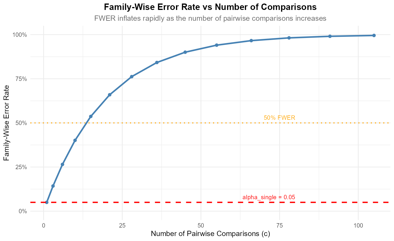
FWER inflation with number of comparisons — Fig. 12.20 **Figure 1**: Family-wise error rate as a function of number of comparisons (α_single = 0.05).

Using Figure 1 or calculations:

Complete the following table showing FWER for different numbers of groups:

k (groups)

c (comparisons)

FWER (α = 0.05)

3

5

10

15
At what number of groups does the FWER first exceed 50%?
A clinical trial compares 6 treatments. If the researchers use individual α = 0.05 tests without correction, approximately what FWER do they face?

Solution

Part (a): Completed table

k (groups)	c (comparisons)	FWER (α = 0.05)
3	3	14.3%
5	10	40.1%
10	45	90.1%
15	105	99.5%

Calculations:

k=3: c = 3, FWER = 1 - 0.95³ = 0.143
k=5: c = 10, FWER = 1 - 0.95¹⁰ = 0.401
k=10: c = 45, FWER = 1 - 0.95⁴⁵ = 0.901
k=15: c = 105, FWER = 1 - 0.95¹⁰⁵ = 0.995

Part (b): FWER exceeds 50%

Solving 1 - 0.95^c ≥ 0.5:

0.95^c ≤ 0.5 → c ≥ log(0.5)/log(0.95) = 13.5

So we need c ≥ 14 comparisons, which first occurs at k = 6 groups (c = 15).

Part (c): Clinical trial with 6 treatments

c = C(6,2) = 15 comparisons

FWER = 1 - 0.95¹⁵ = 1 - 0.463 = 0.537 = 53.7%

More than half the time, they would falsely declare at least one treatment different when no differences exist!

R verification:

# Part (a)
k_values <- c(3, 5, 10, 15)
for (k in k_values) {
  c <- choose(k, 2)
  fwer <- 1 - (0.95)^c
  cat("k =", k, ": c =", c, ", FWER =", round(fwer, 3), "\n")
}

# Part (b)
log(0.5) / log(0.95)  # 13.5
choose(6, 2)  # 15 comparisons at k=6

# Part (c)
1 - 0.95^15  # 0.537

Exercise 3: Bonferroni Correction

A materials scientist compares the hardness of 4 different alloy compositions. After rejecting H₀ in the overall ANOVA F-test, she wants to identify which specific pairs differ.

Given: n = 60 total (15 per group), MSE = 18.5, and the group means are:

Alloy A: x̄₁ = 245.2
Alloy B: x̄₂ = 252.8
Alloy C: x̄₃ = 248.5
Alloy D: x̄₄ = 261.3

Using the Bonferroni correction with overall α = 0.05:

How many pairwise comparisons are there?
What is the adjusted significance level α_single for each comparison?
Calculate the Bonferroni-adjusted critical t-value.
Calculate the confidence interval for μ_D - μ_A.
Is the difference between Alloy D and Alloy A statistically significant?

Exercise 4: Tukey’s HSD Method

Using the same alloy data from Exercise 3, now apply Tukey’s HSD method.

Calculate the Tukey critical value q* using R’s qtukey() function.
Calculate the Tukey-adjusted margin of error for comparing any two groups.
Calculate the Tukey HSD confidence interval for μ_D - μ_A.
Compare the Tukey CI width to the Bonferroni CI width from Exercise 3. Which is narrower?
Why is Tukey’s method generally preferred over Bonferroni for pairwise comparisons?

Exercise 5: Interpreting Tukey HSD Output

A nutritionist compares weight loss (kg) across five diet programs. After a significant ANOVA result, she runs TukeyHSD() in R and obtains:

Tukey multiple comparisons of means
  95% family-wise confidence level

$Diet
            diff     lwr     upr  p adj
B-A        4.20    0.82    7.58  0.0084
C-A       -1.50   -4.88    1.88  0.7123
D-A        6.80    3.42   10.18  0.0000
E-A        3.10   -0.28    6.48  0.0873
C-B       -5.70   -9.08   -2.32  0.0002
D-B        2.60   -0.78    5.98  0.2017
E-B       -1.10   -4.48    2.28  0.8849
D-C        8.30    4.92   11.68  0.0000
E-C        4.60    1.22    7.98  0.0030
E-D       -3.70   -7.08   -0.32  0.0253

Which pairs of diets show statistically significant differences at the 0.05 family-wise level?
Order the diets from lowest to highest mean weight loss.
Create an underline diagram showing which diets are not significantly different.
What practical conclusions can the nutritionist draw?

Exercise 6: Constructing Underline Diagrams

An industrial engineer compares the productivity (units/hour) of workers trained with four different methods. The Tukey HSD results show:

Comparison	Difference	95% CI	Significant?
B - A	2.3	(-0.8, 5.4)	No
C - A	8.5	(5.4, 11.6)	Yes
D - A	5.1	(2.0, 8.2)	Yes
C - B	6.2	(3.1, 9.3)	Yes
D - B	2.8	(-0.3, 5.9)	No
D - C	-3.4	(-6.5, -0.3)	Yes

Order the training methods from lowest to highest mean productivity.
Construct the underline diagram.
Describe the groupings in words.
Which method(s) would you recommend and why?

Exercise 7: Bonferroni vs Tukey Comparison

A researcher compares k = 6 treatment groups with n = 12 observations per group (total n = 72). MSE = 45.0.

Calculate the Bonferroni critical value for 95% family-wise CIs.
Calculate the Tukey critical value for 95% family-wise CIs.
For two groups with means differing by 8.5, calculate both the Bonferroni and Tukey CIs.
Which method would you recommend for this analysis? Why?

Exercise 8: Complete Post-Hoc Analysis

A computer science researcher compares the accuracy (% correct) of 4 machine learning algorithms on a benchmark dataset. Each algorithm is tested on 20 independent runs.

ANOVA Results:

F = 8.72, p-value = 0.00006 (significant at α = 0.05)
MSE = 15.8, df_E = 76

Group Means:

Algorithm A (Random Forest): x̄₁ = 87.3%
Algorithm B (SVM): x̄₂ = 84.1%
Algorithm C (Neural Network): x̄₃ = 91.5%
Algorithm D (Gradient Boosting): x̄₄ = 89.8%

Conduct a complete Tukey HSD analysis:

Calculate the Tukey critical value.
Calculate 95% family-wise CIs for all 6 pairwise differences.
Identify which pairs are significantly different.
Create the underline diagram.
Write a summary of findings for a non-technical audience.

Solution

Assumption Note: Since the ANOVA was already conducted and found significant (p = 0.00006), we assume the standard ANOVA assumptions (independence, normality within groups, equal variances) were verified prior to the analysis. With n = 20 per group and equal sample sizes, ANOVA and Tukey HSD are robust to moderate assumption violations.

Part (a): Tukey critical value

k = 4, df_E = 76, α = 0.05

\[q^* = \frac{q_{0.05, 4, 76}}{\sqrt{2}} = \frac{3.702}{\sqrt{2}} = 2.618\]

Part (b): All pairwise CIs

Standard error (equal n = 20):

\[SE = \sqrt{MSE \cdot \left(\frac{1}{20} + \frac{1}{20}\right)} = \sqrt{15.8 \cdot 0.1} = \sqrt{1.58} = 1.257\]

Margin of error: ME = 2.618 × 1.257 = 3.29

All pairwise comparisons:

Pair	Difference	95% CI	Significant?
B - A	-3.2	(-6.49, 0.09)	No
C - A	4.2	(0.91, 7.49)	Yes
D - A	2.5	(-0.79, 5.79)	No
C - B	7.4	(4.11, 10.69)	Yes
D - B	5.7	(2.41, 8.99)	Yes
D - C	-1.7	(-4.99, 1.59)	No

Part (c): Significant pairs

Significantly different pairs (CI excludes 0):

C - A: Neural Network > Random Forest (by 4.2%)
C - B: Neural Network > SVM (by 7.4%)
D - B: Gradient Boosting > SVM (by 5.7%)

Part (d): Underline diagram

Order by mean: B (84.1) < A (87.3) < D (89.8) < C (91.5)

Non-significant pairs: B-A, A-D, D-C

B ——— A ——— D ——— C
└─────────┘ └─────┘

The two underlines show overlapping groups with no significant difference within each group.

Part (e): Non-technical summary

Summary: Machine Learning Algorithm Comparison

We compared four machine learning algorithms for classification accuracy. Here’s what we found:

Key Finding: The Neural Network algorithm achieved the highest average accuracy (91.5%), which was significantly better than both Random Forest (87.3%) and SVM (84.1%).

Performance Groups:

Top performers: Neural Network (91.5%) and Gradient Boosting (89.8%) - these were not significantly different from each other
Middle performer: Random Forest (87.3%) - overlaps with both top and bottom groups
Lower performer: SVM (84.1%) - significantly worse than Neural Network and Gradient Boosting

Recommendation: For this benchmark task, choose either Neural Network or Gradient Boosting. The Neural Network has a slight edge (1.7% higher) but the difference is not statistically significant. SVM appears to be the weakest choice among these options.

R verification:

k <- 4; n_per <- 20
MSE <- 15.8
df_E <- 76
xbar <- c(87.3, 84.1, 91.5, 89.8)
names(xbar) <- c("A", "B", "C", "D")

# Tukey critical value
q_star <- qtukey(0.05, k, df_E, lower.tail = FALSE) / sqrt(2)  # 2.618

SE <- sqrt(MSE * (1/n_per + 1/n_per))  # 1.257
ME <- q_star * SE  # 3.29

# All pairwise comparisons
pairs <- combn(names(xbar), 2)
for (i in 1:ncol(pairs)) {
  p1 <- pairs[1, i]; p2 <- pairs[2, i]
  diff <- xbar[p2] - xbar[p1]
  ci <- c(diff - ME, diff + ME)
  sig <- ifelse(ci[1] > 0 | ci[2] < 0, "Yes", "No")
  cat(p2, "-", p1, ":", round(diff, 1),
      " CI: (", round(ci[1], 2), ",", round(ci[2], 2), ")",
      " Sig:", sig, "\n")
}

Exercise 9: When NOT to Perform Multiple Comparisons

For each scenario, explain whether multiple comparison procedures should be performed and why.

ANOVA yields F = 1.23, p-value = 0.31
ANOVA yields F = 4.56, p-value = 0.006, but the researcher is only interested in comparing treatments to a control group.
ANOVA yields F = 8.91, p-value < 0.001, comparing 12 different drug formulations.
A study compares only k = 2 groups and finds a significant difference.

12.4.7. Additional Practice Problems

True/False Questions (1 point each)

Multiple comparison procedures should be performed regardless of whether the ANOVA F-test is significant.

Ⓣ or Ⓕ
The Bonferroni correction divides the overall significance level by the number of comparisons.

Ⓣ or Ⓕ
Tukey’s HSD method requires the assumption that all pairwise comparisons are independent.

Ⓣ or Ⓕ
If a Tukey 95% CI for μ_A - μ_B is (-2.5, 4.1), we conclude that A and B are significantly different.

Ⓣ or Ⓕ
The FWER increases as the number of groups increases.

Ⓣ or Ⓕ
Bonferroni correction is more conservative than Tukey’s method for pairwise comparisons.

Ⓣ or Ⓕ

Multiple Choice Questions (2 points each)

An underline diagram shows: A ——— B C ——— D. This indicates:

Ⓐ All four means are significantly different

Ⓑ A differs from C and D; B differs from C and D

Ⓒ Only A-B and C-D pairs are NOT significantly different

Ⓓ The ANOVA F-test was not significant
Which method is specifically designed for comparing treatments to a control?

Ⓐ Bonferroni

Ⓑ Tukey HSD

Ⓒ Dunnett

Ⓓ Šidák
The Tukey critical value is obtained from which distribution?

Ⓐ t-distribution

Ⓑ F-distribution

Ⓒ Studentized range distribution

Ⓓ Chi-square distribution