Slides 📊

Download Chapter 7 slides (PPTX)

7.1. Statistics and Sampling Distributions

We’ve spent considerable time building probability models that describe populations. Now we reach a pivotal moment in our statistical journey: the bridge from probability theory to statistical inference. This transition first requires the understanding of how sample statistics themselves behave as random variables.

Road Map 🧭

• Understand how sample statistics can be viewed as random variables.

• Master the theoretical properties of sample statistics in relation to the population distribution.

7.1.1. Parameters, Statistics, and Estimators

Population Parameters

Recall that a parameter is a number that describes some attribute of the population. For example, the population mean \(\mu\) is a parameter that tells us the average value across all units in the population. We often study the theoretical behavior of probability distributions assuming that we know these parameters. But in statistical inference, the tables turn—parameters are usually unknown, and we try to learn about them through observed samples. However, we should always keep in mind that, though unknown, the parameters always exist as fixed, non-random values.

Sample Statistics: Our Window Into the Population

A statistic \(T\) is a function that maps each sample to a numerical summary \(t\):

\[T(x_1, x_2, \cdots, x_n) = t\]

One example is the sample mean \(\bar{x} = \frac{1}{n}\sum_{i=1}^n x_i\), which summarizes the center of an observed sample. Unlike parameters, we can calculate statistics directly from the data.

The crucial insight is that statistics will change from sample to sample. If we collect multiple samples of the same size from the same population, we will almost certainly get different values of \(\bar{x}\) from all the samples.

Estimators: Statistics with a Purpose

An estimator is a statistic which targets a specific population parameter. We use the sample mean \(\bar{x}\) as an estimator of the population mean \(\mu\). We use the sample standard deviation \(s\) as an estimator of the population standard deviation \(\sigma\).

The sample mean \(\bar{x}\) is both a statistic (it summarizes the sample) and an estimator (it targets the population mean \(\mu\)). This dual role of a data summary is key to statistical inference, since it has significance for both the sample and the population. It not only describes the observed data but also provides a basis for drawing conclusions about the underlying distribution.

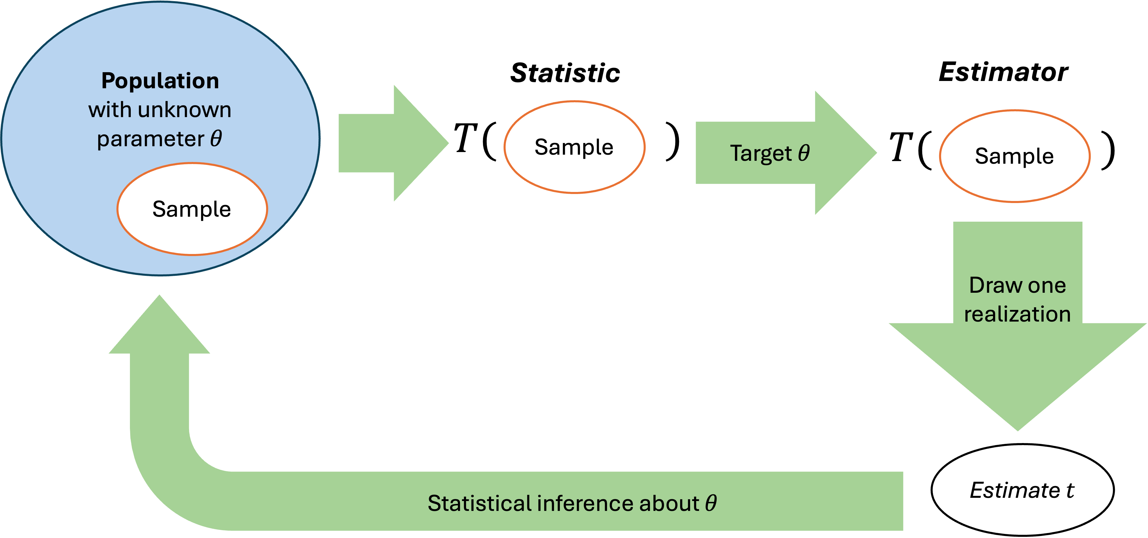
Fig. 7.1 Parameters describe the population; statistics summarize the sample; estimators target the unknown parameters

7.1.2. The Sampling Distribution

To understand how estimators behave across many possible samples, we must establish the concept of a sampling distribution.

The Thought Experiment

Suppose we are studying the heights of college students and we have enough resources to replicate the study many times. During each single run of the study, we take a sample of size \(n = 25\). We collect our first sample, measure all \(25\) students, and compute \(\bar{x}_1 = 67.2\) inches. We collect a second sample of \(25\) different students and get \(\bar{x}_2 = 68.8\) inches. A third sample gives \(\bar{x}_3 = 66.9\) inches.

If we repeated this process thousands of times, we would have thousands of different sample means: \(\bar{x}_1, \bar{x}_2, \cdots, \bar{x}_m\). These sample means would vary, and that variation would follow a pattern. The distribution of these sample means is called the sampling distribution of the sample mean.

Formal Definition

The sampling distribution of a statistic is the probability distribution of that statistic across all possible samples of the same size from the same population. It tells us how the statistic behaves as a random variable.

This concept applies to any statistic—sample means, sample standard deviations, sample medians, sample correlations. Each has its own sampling distribution that describes how that particular statistic varies from sample to sample.

Why This Matters for Inference

Understanding sampling distributions allows us to quantify the uncertainty in our estimates. If we know how \(\bar{X}\) behaves across many samples, we can assess how reliable any single observed \(\bar{x}\) might be as an estimate of \(\mu\). This knowledge forms the foundation for confidence intervals, hypothesis tests, and all other inferential procedures.

The Capital \(\bar{X}\)

We will now study the behavior of sample statistics as random variables. To distinguish from contexts where they serve as realized values, we use capital letters. \(\bar{X}\) denotes the random variable that generates \(\bar{x}\)’s. Similar distinctions apply to \(S\) vs. \(s\) and \(S^2\) vs. \(s^2\).

7.1.3. Factors Affecting Sampling Distributions

1. The population distribution

2. Sample size, \(n\)

3. The statistic itself

   For example, \(S\) can only take positive values, while \(\bar{X}\) has no such restriction. This is due to the difference in how the two statistics are defined.

4. The sampling technique

   The sampling technique affects how well a sample represents the population and whether key properties like independence are satisfied.

We will examine how these factors influence inference in greater depth in the upcoming chapters.

7.1.4. Bringing It All Together

Key Takeaways 📝

1. Statistics are random variables that vary from sample to sample, creating sampling distributions that describe this variability. Understanding how statistics behave as random variables lets us quantify uncertainty and make conclusions about unknown populations.

2. Sampling distributions are determined by multiple factors. The population distribution, sample size, the choice of statistic, and independence all play important roles.

7.1.5. Exercises

These exercises develop your conceptual understanding of the distinction between parameters and statistics, the role of estimators, and the fundamental concept of sampling distributions.

Key Terminology

• Parameter: A fixed (but often unknown) numerical value describing a population (e.g., μ, σ, p)

• Statistic: A numerical summary computed from sample data; formally, a function \(T(x_1, x_2, \ldots, x_n) = t\) that maps a sample to a number. For example, \(T\) could be the sample mean, in which case \(T(x_1, \ldots, x_n) = \bar{x}\).

• Estimator: A statistic used to estimate a specific population parameter

• Sampling distribution: The probability distribution of a statistic across all possible samples of the same size

Exercise 1: Parameter vs. Statistic Identification

For each of the following, identify whether the quantity described is a parameter or a statistic. Justify your answer.

1. The average GPA of all 45,000 undergraduate students at Purdue University.

2. The average GPA computed from a random sample of 200 Purdue undergraduates.

3. The proportion of all registered voters in Indiana who support a particular policy.

4. In a survey of 1,500 Indiana voters, 58% indicated support for the policy.

5. The standard deviation of response times for all requests processed by a web server in 2024.

6. The standard deviation computed from a log of 500 randomly selected server requests.

Solution

Part (a): Parameter

This describes the average for the entire population of Purdue undergraduates (all 45,000). It is a fixed value, even if unknown or difficult to compute.

Part (b): Statistic

This is computed from sample data (200 students). It will vary depending on which 200 students are selected.

Part (c): Parameter

This describes a characteristic of the entire population of Indiana voters. It is a fixed proportion, denoted \(p\).

Part (d): Statistic

The 58% is computed from sample data (1,500 voters). It is an estimate of the population proportion, denoted \(\hat{p} = 0.58\).

Part (e): Parameter

This is the standard deviation for all requests in 2024—the entire population of interest. It is denoted \(\sigma\).

Part (f): Statistic

This is computed from a sample of 500 requests. It is denoted \(s\) and serves as an estimate of \(\sigma\).

---

Exercise 2: Estimators and Their Targets

Match each estimator (statistic) with the population parameter it targets.

Estimator (Statistic)	Population Parameter
Sample mean \(\bar{x}\)	Population variance \(\sigma^2\)
Sample standard deviation \(s\)	Population proportion \(p\)
Sample variance \(s^2\)	Population mean \(\mu\)
Sample proportion \(\hat{p}\)	Population standard deviation \(\sigma\)

Solution

• A → 3: Sample mean \(\bar{x}\) estimates population mean \(\mu\)

• B → 4: Sample standard deviation \(s\) estimates population standard deviation \(\sigma\)

• C → 1: Sample variance \(s^2\) estimates population variance \(\sigma^2\)

• D → 2: Sample proportion \(\hat{p}\) estimates population proportion \(p\)

---

Exercise 3: Understanding Sampling Variability

A pharmaceutical company wants to estimate the mean reduction in blood pressure (mmHg) for patients taking a new medication. They conduct three separate studies, each with a random sample of 50 patients from the same population.

• Study 1: \(\bar{x}_1 = 8.2\) mmHg

• Study 2: \(\bar{x}_2 = 7.6\) mmHg

• Study 3: \(\bar{x}_3 = 8.9\) mmHg

1. Why did the three studies produce different sample means?

2. If the company conducted 1,000 such studies (each with n = 50), what would the distribution of the 1,000 sample means be called?

3. Is the population mean \(\mu\) equal to 8.2, 7.6, or 8.9? Explain.

4. Which of the following would reduce the variability among sample means: increasing sample size to n = 200, or conducting more studies with n = 50?

Solution

Part (a): Sampling variability

The three studies produced different sample means because each study used a different random sample of 50 patients. Even though all samples came from the same population, random sampling introduces variability—different patients happen to be selected, and they have different responses to the medication.

Part (b): Sampling distribution

The distribution of the 1,000 sample means is called the sampling distribution of the sample mean (or sampling distribution of \(\bar{X}\)).

Part (c): The population mean μ

We cannot say that \(\mu\) equals any of these values. The population mean \(\mu\) is a fixed but unknown parameter. The values 8.2, 7.6, and 8.9 are statistics—estimates of \(\mu\) that vary from sample to sample. The true \(\mu\) might be close to these values, but it is not necessarily equal to any of them.

Part (d): Reducing variability

Increasing the sample size to n = 200 would reduce the variability among sample means. Larger samples provide more information about the population and result in sample means that cluster more tightly around the true population mean.

Conducting more studies with n = 50 would give us more sample means to observe, but each individual sample mean would still have the same variability. More studies help us see the sampling distribution better, but they don’t make individual estimates more precise.

---

Exercise 4: The Sampling Distribution Concept

Consider a population of 5 employees with the following annual salaries (in thousands of dollars): 45, 50, 55, 60, 70.

1. Calculate the population mean \(\mu\) and population standard deviation \(\sigma\).

2. List all possible samples of size n = 2 (sampling without replacement). How many are there?

3. For each sample, calculate the sample mean \(\bar{x}\).

4. Create the sampling distribution of \(\bar{X}\) by listing each possible value and its probability.

5. Calculate the mean of the sampling distribution. How does it compare to \(\mu\)?

Solution

Part (a): Population parameters

Population: {45, 50, 55, 60, 70}

\[\mu = \frac{45 + 50 + 55 + 60 + 70}{5} = \frac{280}{5} = 56 \text{ thousand dollars}\]

\[\sigma^2 = \frac{(45-56)^2 + (50-56)^2 + (55-56)^2 + (60-56)^2 + (70-56)^2}{5}\]

\[= \frac{121 + 36 + 1 + 16 + 196}{5} = \frac{370}{5} = 74\]

\[\sigma = \sqrt{74} = 8.602 \text{ thousand dollars}\]

Part (b): All possible samples of size 2

The number of samples is \(\binom{5}{2} = 10\).

The samples are: {45,50}, {45,55}, {45,60}, {45,70}, {50,55}, {50,60}, {50,70}, {55,60}, {55,70}, {60,70}.

Part (c): Sample means

Sample	\(\bar{x}\)
{45, 50}	47.5
{45, 55}	50.0
{45, 60}	52.5
{45, 70}	57.5
{50, 55}	52.5
{50, 60}	55.0
{50, 70}	60.0
{55, 60}	57.5
{55, 70}	62.5
{60, 70}	65.0

Part (d): Sampling distribution of \(\bar{X}\)

Each sample is equally likely with probability 1/10.

\(\bar{x}\)	\(P(\bar{X} = \bar{x})\)
47.5	1/10
50.0	1/10
52.5	2/10
55.0	1/10
57.5	2/10
60.0	1/10
62.5	1/10
65.0	1/10

Part (e): Mean of the sampling distribution

\[E[\bar{X}] = 47.5(0.1) + 50.0(0.1) + 52.5(0.2) + 55.0(0.1) + 57.5(0.2)\]

\[+ 60.0(0.1) + 62.5(0.1) + 65.0(0.1)\]

\[= 4.75 + 5.0 + 10.5 + 5.5 + 11.5 + 6.0 + 6.25 + 6.5 = 56\]

The mean of the sampling distribution equals the population mean: \(E[\bar{X}] = \mu = 56\).

This is not a coincidence—it is always true that \(E[\bar{X}] = \mu\). The sample mean is an unbiased estimator of the population mean.

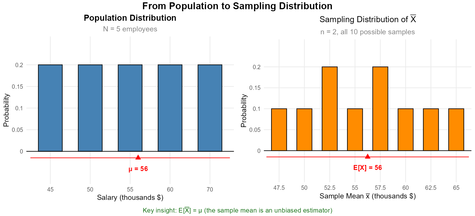
Fig. 7.2 Left: The population distribution (5 salaries). Right: The sampling distribution of X̄ for samples of size 2. Notice that E[X̄] = μ = 56, but the sampling distribution is more concentrated (less spread) than the population.

---

Exercise 5: Notation and Random Variables

Explain the distinction between each pair of symbols. When would you use each?

1. \(\mu\) vs. \(\bar{x}\)

2. \(\bar{X}\) vs. \(\bar{x}\)

3. \(\sigma\) vs. \(s\)

4. \(S^2\) vs. \(s^2\)

Solution

Part (a): μ vs. x̄

• \(\mu\) is the population mean—a fixed parameter describing the center of the entire population.

• \(\bar{x}\) is the sample mean—a statistic computed from observed sample data.

Use \(\mu\) when referring to the true (but possibly unknown) population average. Use \(\bar{x}\) when reporting the average of your observed sample.

Part (b): X̄ vs. x̄

• \(\bar{X}\) (capital) is the sample mean treated as a random variable—before any specific sample is collected. It has a sampling distribution.

• \(\bar{x}\) (lowercase) is a realized value—the specific numerical result after collecting data.

Use \(\bar{X}\) when discussing the theoretical properties of the sample mean (e.g., “the sampling distribution of \(\bar{X}\)”). Use \(\bar{x}\) when reporting the result from actual data (e.g., “we observed \(\bar{x} = 52.3\)”).

Part (c): σ vs. s

• \(\sigma\) is the population standard deviation—a fixed parameter.

• \(s\) is the sample standard deviation—a statistic computed from sample data.

Use \(\sigma\) when the population SD is known or when referring to the true population variability. Use \(s\) when you’ve calculated SD from sample data.

Part (d): S² vs. s²

• \(S^2\) (capital) is the sample variance as a random variable—its value depends on which sample is drawn.

• \(s^2\) (lowercase) is the computed sample variance from a specific observed sample.

Use \(S^2\) when discussing theoretical properties. Use \(s^2\) when reporting a calculated value.

---

Exercise 6: Factors Affecting Sampling Distributions

For each scenario, identify which factor(s) affecting the sampling distribution are relevant: (i) population distribution, (ii) sample size, (iii) the statistic itself, or (iv) sampling technique (which governs independence and potential bias).

1. Increasing the sample size from n = 30 to n = 100 makes sample means cluster more tightly around the population mean.

2. The sampling distribution of the sample median has a different shape than the sampling distribution of the sample mean.

3. A convenience sample (surveying only friends) produces biased estimates of population parameters.

4. When the population is highly skewed, small samples produce sample means with skewed sampling distributions.

5. The sample standard deviation \(S\) can only take non-negative values, while the sample mean \(\bar{X}\) can be any real number.

Solution

Part (a): Sample size (ii)

Larger samples provide more information, reducing the variability (spread) of the sampling distribution.

Part (b): The statistic itself (iii)

Different statistics (mean vs. median) have different sampling distributions, even when applied to the same population and sample size.

Part (c): Sampling technique (iv)

Non-random sampling methods (like convenience sampling) can introduce bias and violate independence assumptions. The sampling technique governs both whether observations are independent and whether the sample is representative of the population.

Part (d): Population distribution (i)

The shape of the population affects the sampling distribution, especially for small samples. For large samples, the Central Limit Theorem (covered in Section 7.3) helps make the sampling distribution approximately normal regardless of population shape.

Part (e): The statistic itself (iii)

The definition of the statistic determines its possible values. Standard deviation is defined as a non-negative quantity, while the mean has no such restriction.

---

Exercise 7: Conceptual Scenarios

Determine whether each statement is true or false. Explain your reasoning.

1. If we know the population mean \(\mu\), then the sample mean \(\bar{x}\) will always equal \(\mu\).

2. Different samples from the same population will generally produce different sample statistics.

3. The population parameter \(\mu\) is a random variable that changes from sample to sample.

4. The sampling distribution describes how a statistic varies across all possible samples.

5. If sample size increases, the sampling distribution of \(\bar{X}\) becomes more spread out.

6. An estimator is a special type of statistic that targets a specific population parameter.

Solution

Part (a): False

The sample mean \(\bar{x}\) is subject to sampling variability. It will typically be close to \(\mu\) but will rarely equal it exactly. Only in the trivial case where the sample includes the entire population would we expect \(\bar{x} = \mu\).

Part (b): True

Due to sampling variability, different samples contain different observations, leading to different computed statistics.

Part (c): False

Parameters are fixed values that describe the population. They do not change. It is the statistics that are random variables varying from sample to sample.

Part (d): True

This is the definition of a sampling distribution—it describes the probability distribution of a statistic across all possible samples of a given size.

Part (e): False

As sample size increases, the sampling distribution becomes less spread out (more concentrated around the true parameter). Larger samples yield more precise estimates.

Part (f): True

An estimator is indeed a statistic used specifically to estimate a population parameter. For example, \(\bar{x}\) is both a statistic (it summarizes the sample) and an estimator (it targets \(\mu\)).

---

7.1.6. Additional Practice Problems

True/False Questions (1 point each)

1. A parameter is a numerical summary of sample data.

   Ⓣ or Ⓕ

2. The sample mean \(\bar{X}\) is a random variable.

   Ⓣ or Ⓕ

3. Different random samples from the same population will produce the same sample mean.

   Ⓣ or Ⓕ

4. The sampling distribution of a statistic describes how that statistic varies across all possible samples.

   Ⓣ or Ⓕ

5. The population standard deviation \(\sigma\) changes depending on which sample is selected.

   Ⓣ or Ⓕ

6. An estimator is a statistic used to estimate a population parameter.

   Ⓣ or Ⓕ

Multiple Choice Questions (2 points each)

7. Which of the following is a parameter?

   Ⓐ The average height of 50 randomly selected students

   Ⓑ The standard deviation of test scores for all students in a school

   Ⓒ The sample proportion of defective items in a shipment

   Ⓓ The median income from a survey of 1,000 households

8. The sampling distribution of the sample mean describes:

   Ⓐ How individual observations vary within a single sample

   Ⓑ How the sample mean varies across all possible samples

   Ⓒ The shape of the population distribution

   Ⓓ The relationship between sample size and population size

9. Which symbol represents the sample mean as a random variable?

   Ⓐ \(\mu\)

   Ⓑ \(\bar{x}\)

   Ⓒ \(\bar{X}\)

   Ⓓ \(\sigma\)

10. What happens to the sampling distribution of \(\bar{X}\) as sample size increases?

    Ⓐ It becomes more spread out

    Ⓑ It becomes less spread out (more concentrated)

    Ⓒ It shifts to the right

    Ⓓ It remains unchanged

11. The sample standard deviation \(s\) is used as an estimator of:

    Ⓐ \(\mu\)

    Ⓑ \(\bar{x}\)

    Ⓒ \(\sigma\)

    Ⓓ \(n\)

12. Which of the following is NOT a factor that affects sampling distributions?

    Ⓐ The population distribution

    Ⓑ The sample size

    Ⓒ The color of the data collection forms

    Ⓓ The choice of statistic

Answers to Practice Problems

True/False Answers:

1. False — A parameter describes the population, not the sample. A statistic summarizes sample data.

2. True — Before data is collected, \(\bar{X}\) is a random variable whose value depends on which sample is drawn.

3. False — Different samples will generally produce different sample means due to sampling variability.

4. True — This is the definition of a sampling distribution.

5. False — Population parameters like \(\sigma\) are fixed values. They do not depend on the sample.

6. True — An estimator is a statistic with the specific purpose of estimating a population parameter.

Multiple Choice Answers:

7. Ⓑ — “All students in a school” indicates this is a population characteristic, making it a parameter. The others are computed from samples.

8. Ⓑ — The sampling distribution describes how the statistic (sample mean) varies across all possible samples of the same size.

9. Ⓒ — Capital \(\bar{X}\) denotes the sample mean as a random variable. Lowercase \(\bar{x}\) is a realized value, and \(\mu\) is the population mean.

10. Ⓑ — Larger samples produce sample means that are more tightly clustered around the population mean, reducing the spread of the sampling distribution.

11. Ⓒ — The sample standard deviation \(s\) estimates the population standard deviation \(\sigma\).

12. Ⓒ — The color of forms has no statistical relevance. Population distribution, sample size, and choice of statistic all affect sampling distributions.