Slides 📊

11.4. Independent Two-Sample Analysis - No Equal Variance Assumption

When population standard deviations are unknown and we cannot reasonably assume that the variances are equal across populations, each variance must be estimated separately. This section develops the unpooled approach for indepndent two-sample comparisons and emphasizes the importance of choosing the appropriate method—pooled or unpooled—based on evidence provided by the data.

Road Map 🧭

Estimate the standard error for independent two-sample comparison without the equal variance assumption.
Recognize that the new pivotal method approximately follows a \(t\)-distribution and that its degrees of freedom must also be approximated.
Use Welch-Satterthwaite approximation for the degrees of freedom.
Learn the consequences of incorrectly using the pooled versus unpooled approaches and why it is safer to use the more general unpooled approach as the default.
Know that the unpooled procedure is robust to moderate departures from normality. List the characteristics of the data for which we expect the method to work best.

11.4.1. Mathematical Framework

The Assumptions

This lesson still develops upon the core assumptions introduced in Chapter 11.2.1.

Recall the true standard error for the difference of means \(\bar{X}_A - \bar{X}_B\):

\[\sigma_{\bar{X}_A - \bar{X}_B} = \sqrt{\frac{\sigma^2_A}{n_A} + \frac{\sigma^2_B}{n_B}}.\]

Since the two population variance \(\sigma^2_A\) and \(\sigma^2_B\) are not assumed equal anymore, we do not take any further simplification steps and directly replace the unknown values with their respective estimators, \(S^2_A\) and \(S^2_B\).

The estimated standard error is then:

\[\widehat{SE} = \sqrt{\frac{S^2_A}{n_A} + \frac{S^2_B}{n_B}}.\]

It follows that the studentization of \(\bar{X}_A - \bar{X}_B\) is:

(11.3)\[T' = \frac{(\bar{X}_A - \bar{X}_B) - (\mu_A -\mu_B)}{\sqrt{\frac{S^2_A}{n_A} + \frac{S^2_B}{n_B}}}.\]

The pivotal quantity is denoted \(T'\) with a prime because even when all assumptions hold, it only approximately follows a \(t\)-distribution. Not only that, the true degrees of freedom for the best approximating \(t\)-distribution depends on the unknown variances and must also be approximated.

We use the Welch-Satterthwaite Approximation for the unknown degrees of freedom:

\[\nu = \frac{\left(\frac{s^2_A}{n_A} + \frac{s^2_B}{n_B}\right)^2}{\frac{1}{n_A - 1}\left(\frac{s^2_A}{n_A}\right)^2 + \frac{1}{n_B - 1}\left(\frac{s^2_B}{n_B}\right)^2}\]

Once \(\nu\) is computed, we treat \(T'\) as having a \(t\)-dstribution with the degrees of freedom \(\nu\) for further construction of inference methods. This approximation generally shows good performance in practice—it tends to produce a slightly conservative inference result (wider confidence regions, less likely to reject \(H_0\)) when sample sizes are small.

The Approximated \(\nu\) May Not Be an Integer

\(\nu\) is typically not integer-valued, which is okay. R accepts non-integer values for the df argument of \(t\)-related functions. Use the approximated \(\nu\) without making any adjustments.

11.4.2. Hypothesis Tests and Confidence Regions

Hypothesis Testing

Within the four-step framework of hypothesis testing, Steps 1, 2, and 4 of the unpooled approach is identical to the other types of independent two-sample comparisons. Revisit Chapter 11.2 for the related details. We will focus on Step 3, where we compute the test statistic, degrees of freedom, and p-value.

The observed test statistic takes the familiar form: it is the difference between the observed point estimate and the null value, standardized by the estimated standard error.

\[t'_{TS} = \frac{(\bar{x}_A - \bar{x}_B) - \Delta_0}{\sqrt{\frac{s^2_A}{n_A} + \frac{s^2_B}{n_B}}}\]

Compute the degrees of freedom \(\nu\) using the Welch-Satterthwaite Approximation formula. Then the \(p\)-values are:

Two-sided: \(2P(T_\nu < -|t'_{TS}|)\)
Upper-tailed: \(P(T_\nu > |t'_{TS}|)\)
Left-tailed: \(P(T_\nu < -|t'_{TS}|)\)

Example 💡: Teaching Methods Comparison

To investigate whether directed reading activities improve students’ reading ability, students at an elementary school were randomly assigned to either directed reading activities or standard instruction.

Their performance was measured by Degree of Reading Power (DRP) scores. Higher DRP scores indicate better reading ability. The observed statistics are:

Method	New	Standard
Sample size	\(n_{new} = 21\)	\(n_{std} = 23\)
Sample mean	\(\bar{x}_{new} = 51.48\)	\(\bar{x}_{std} = 41.52\)
Sample standard deviation	\(s_{new} = 11.01\)	\(s_{std} = 17.15\)

Step 1: Define Parameters

Use \(\mu_{new}\) to denote the true mean DRP score for students receiving directed reading instruction and \(\mu_{std}\) for the true mean DRP score for students receiving traditional instruction.

Both population standard deviations are unknown and will be estimated separately.

Step 2: Formulate Hypothesis

\[\begin{split}&H_0: \mu_{new} - \mu_{std} \leq 0\\ &H_a: \mu_{new} - \mu_{std} > 0\end{split}\]

Step 3-1: Explore Data and Choose Analysis Method

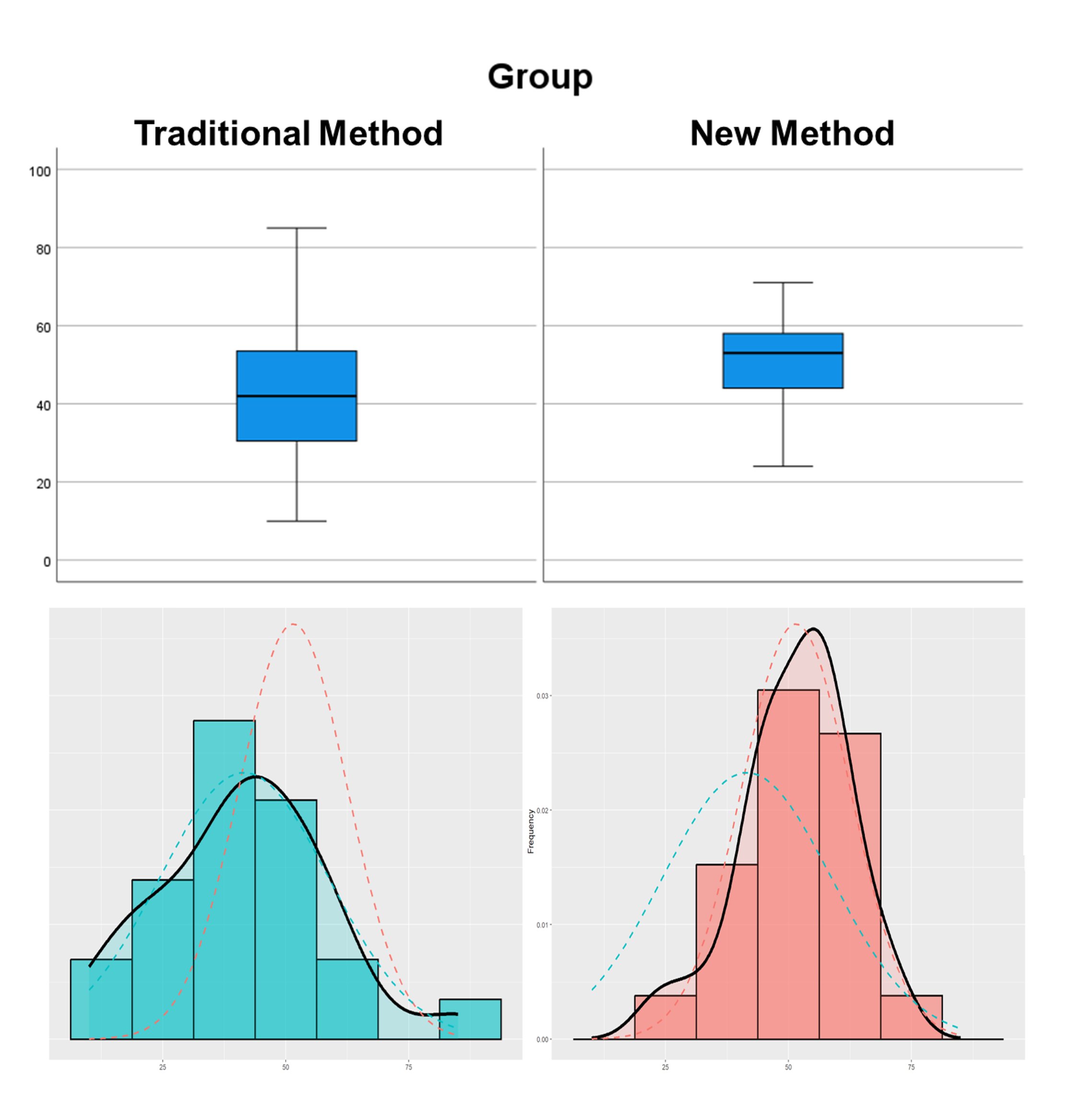
Boxplots and histograms by groups — Fig. 11.6 Boxplots and historgrams by groups

Both distributions approximately normal with mild skewness in the traditional group. Sample sizes are adequate for mild departures from normality.
No serious outliers identified in modified box plots.
Some evidence that variances may differ between groups.

We use the unpooled indpendent two-sample approach.

Step 3-2: Computate Test Statistic, DF, and p-Value

The observed test statistic is:

\[t'_{TS} = \frac{(51.48 - 41.52) - 0}{\sqrt{\frac{11.01^2}{21} + \frac{17.15^2}{23}}} = \frac{9.96}{\sqrt{5.77 + 12.78}} = \frac{9.96}{4.31} = 2.31\]

For the Welch-Satterthwaite approximate degrees of freedom, we encourage breaking down its computation into small components.

\(\frac{s^2_{new}}{n_{new}} = \frac{11.01^2}{21}=5.77\)
\(\frac{s^2_{std}}{n_{std}} = \frac{17.15^2}{23}=12.78\)

Then finally,

\[\nu = \frac{\left(5.77 + 12.78\right)^2}{\frac{5.77^2}{20} + \frac{12.78^2}{22}} = \frac{343.25}{\frac{33.29}{20} + \frac{163.33}{22}} = \frac{343.25}{1.66 + 7.42} = 37.8\]

The \(p\)-value is \(P(T_{37.8} > 2.31)\). Using R,

pt(2.31, df = 37.8, lower.tail = FALSE)

\(p\)-value \(=0.013\).

Step 4: Write the Decision and Conclusion

Since p-value \(= 0.013 < \alpha = 0.05\), we reject the null hypothesis. The data give some support (p-value = 0.013) to the claim that directed reading activities improve elementary school students’ reading ability as measured by DRP scores.

11.4.3. Confidence Regions

The confidence regions can be derived using the pivotal method and \(T'\) in Eq. (11.3).

Confidence regions for independent two-sample tests (unknown unpooled variances)
Confidence interval	\[(\bar{x}_A - \bar{x}_B) \pm t_{\alpha/2,\nu} \sqrt{\frac{s^2_A}{n_A} + \frac{s^2_B}{n_B}}\]
Upper confidence bound	\[(\bar{x}_A - \bar{x}_B) + t_{\alpha,\nu} \sqrt{\frac{s^2_A}{n_A} + \frac{s^2_B}{n_B}}\]
Lower confidence bound	\[(\bar{x}_A - \bar{x}_B) - t_{\alpha,\nu} \sqrt{\frac{s^2_A}{n_A} + \frac{s^2_B}{n_B}}\]

The critical value \(t_{\alpha/2,\nu}\) (or \(t_{\alpha,\nu}\)) is computed with \(\nu\) approximated using the Welch-Satterthwaite formula.

Example 💡: Teaching Methods Comparison, Continued

For the teaching methods comparison problem, compute the confidence region consistent with the previously performed hypothesis test. The summary statistics are:

Method	New	Standard
Sample size	\(n_{new} = 21\)	\(n_{std} = 23\)
Sample mean	\(\bar{x}_{new} = 51.48\)	\(\bar{x}_{std} = 41.52\)
Sample standard deviation	\(s_{new} = 11.01\)	\(s_{std} = 17.15\)

95% Lower Confidence Bound

An upper-tailed hypothesis test is consistent with a lower confidence bound as long as the significance level and the confidence coefficient add to one. Therefore, we need to compute a 95% lower confidence bound for the difference \(\mu_{new} - \mu_{std}.\) From the previous example, we already have

Observed sample difference: \(\bar{x}_{new} - \bar{x}_{std} = 9.96\)
Estimated standard error: \(\widehat{SE} = 4.31\)
The Welch-Satterthwaite approximate degrees of freedom: \(\nu = 37.8\)

The critical value for a one-sided confidence region is

qt(0.05, df=37.8, lower.tail=FALSE)
#returns 1.686

Finally, the lower bound is:

\[9.96 - 1.686(4.31) = 9.96 - 7.27 = 2.69\]

We are 95% confident that the new teaching method improves DRP scores by more than 2.69 points on average.

Using t.test() Function fo Inferences

When we have the complete raw data, we can use t.test() to perform a hypothesis test and compute a confidence region simultaneously.

First, organize the data into two vectors.

The vector quantitiativeVariable should list all observations from both groups.
The vector categoricalVariable should list the group labels of the observations listed in the quantitativeVariable vector.

Then run the following code after replacing each argument with the appropriate values:

t.test(quantitativeVariable ~ categoricalVariable,
      mu = Delta0,
      conf.level = C,
      paired = FALSE,
      alternative = "alternative_hypothesis",
      var.equal = FALSE)

For the teaching methods comparison problem, we would set

mu=0
conf.level = 0.95
paired=FALSE (Paired two-sample analysis if TRUE)
alternative="greater" (other options are two.sided and less)
var.equal=FALSE (Pooled if TRUE; Unpooled is the default choice for this course)

11.4.4. Pooled vs Unpooled Approaches

When choosing between the pooled and unpooled approaches, it is preferable to use the method that best reflects the truth. If the population variances are indeed equal, the pooled method is more appropriate; otherwise, the unpooled approach should be used. However, since the true variances are typically unknown, this simple rule is often impractical to apply.

Let us examine the consequences of incorrectly using pooled versus unpooled methods and explain why we adopt the unpooled approach as the default choice in this course.

Incorrectly Using the Unpooled Approach

By using the unpooled approach for two populations whose variances are in fact equal, we lose efficiency in two aspects:

The analysis method becomes unnecessarily complicated. Instead of the exact \(t\)-distribution and the simple, integer-valued degrees of freedom \(df=n_A + n_B -2,\) we must use the approximation method.
The approach uses the data points less efficiently, leading to decreased power.

Note that incorrectly applying a more general (unpooled) method to a special case (equal true variances) leads to some loss in efficiency but rarely leads to serious errors.

Incorrectly using the Pooled Approach

The consequences are typically more serious when a special-case method is applied incorrectly to a general case. Using a pooled approach on samples drawn from populations with unequal variances risks not only a loss of efficiency but also a loss of theoretical validity.

The problem is especially pronounced when the two sample sizes differ substantially. Consider a scenario where \(n_A = 1500\), \(n_B = 200\). The pooled variance estimator becomes:

\[S^2_p = \frac{(1499)S^2_A + (199)S^2_B}{1697}\]

Since \(n_A\) is much larger than \(n_B\), the pooled estimator will be heavily weighted toward \(S^2_A\).

When \(\sigma_A > \sigma_B\)

If \(\sigma_A > \sigma_B\), then the overall variability will be overestimated, leading to:

Overly wide confidence intervals, and
Reduced power—true differences become harder to detect.

When \(\sigma_A < \sigma_B\)

On the other hand, if \(\sigma_A < \sigma_B\), then the overall variability will be underestimated. As a result,

Confidence interals become too narrow and fail to contain the true difference with the nominal \(100C \%\) coverage probability; the true coverage probability will be smaller.
The hypothesis tests will have type I error rate greater than \(\alpha\); that is, the test will make the mistake more often than \(100\alpha \%\) of the time.

The consequences are especially severe when the true variability is underestimated, as the resulting inferences no longer satisfy the theoretical guarantees they are intended to uphold.

The Unpooled Method is the Default in this Course‼️

Unless directed otherwise, students are expected to solve indpendent two-sample inference problems with unkown variances using the unpooled approach.

11.4.5. Robustness and Assumption Checking

The unpooled \(t\)-procedure is robust to moderate departures from normality, with robustness increasing with sample size. Use the following guidelines on the sample sizes and types of departure from normality.

A. Sample Size Guidelines

Total Sample Size	Normality Requirements
\(n_A + n_B < 15\)	Data must be very close to normal. Requires careful graphical assessment.
\(15 \leq n_A + n_B < 40\)	Can tolerate mild skewness. Strong skewness still problematic.
\(n_A + n_B \geq 40\)	Usually acceptable even with moderate skewness.

When \(n_A \approx n_B\), t-procedures are more robust to moderate normality violations.

B. Guidelines on Different Types of Departure from Normality

In addition to the total sample size, the robustness of \(t\)-procedures also depends on the specific nature of departure from normality. Visualize the data using histograms, QQ plots, and side-by-side boxplots.

Outliers can invalidate procedures regardless of sample size
Extreme skewness or heavy tails may require much larger samples than guidelines suggest
Multiple modes may indicate population heterogeneity

11.4.6. Bringing It All Together

Key Takeaways 📝

Unpooled procedures avoid the restrictive equal variance assumption by estimating the standard error with \(\widehat{SE} = \sqrt{\frac{S^2_A}{n_A} + \frac{S^2_B}{n_B}}\).
The distribution of the pivotal quantity \(T'\) must be approximated with a \(t\)-distribution. We use the Welch-Satterthwaite approximation for its approximate degrees of freedom.
Pooled procedures can result in serious failures when equal variance assumptions are violated.
Unpooled procedures provide robust inference that works whether variances are equal or unequal, with only minor efficiency loss when variances are actually equal. This course uses the unpooled procedure as the default independent two-sample method.

11.4.7. Exercises

Exercise 1: Welch-Satterthwaite Degrees of Freedom

Two independent samples have the following characteristics:

Sample A: \(n_A = 15\), \(s^2_A = 28.4\)
Sample B: \(n_B = 20\), \(s^2_B = 45.7\)

Calculate the Welch-Satterthwaite degrees of freedom \(\nu\).
Compare this to the pooled degrees of freedom \(n_A + n_B - 2\).
Explain why the Welch df is typically smaller than the pooled df.
How does the Welch df change if the sample variances were equal (\(s^2_A = s^2_B = 37\))?

Exercise 2: Computing the Unpooled Standard Error

For each scenario, calculate the unpooled (Welch) estimated standard error.

\(n_A = 20\), \(s_A = 8\), \(n_B = 25\), \(s_B = 10\)
\(n_A = 12\), \(s_A = 15\), \(n_B = 30\), \(s_B = 6\)
Compare the unpooled SE from part (b) to what the pooled SE would be if equal variances were assumed.

Exercise 3: Unpooled Two-Tailed t-Test

A computer scientist compares algorithm execution times (milliseconds) on two different processors.

Processor A: \(n_A = 18\), \(\bar{x}_A = 125\), \(s_A = 22\)
Processor B: \(n_B = 24\), \(\bar{x}_B = 140\), \(s_B = 35\)

Test whether the mean execution times differ at α = 0.05 using the unpooled method.

Exercise 4: Unpooled Upper-Tailed t-Test

A teaching effectiveness study compares student performance with two instructional methods. The variances are not assumed equal.

Method A (active learning): \(n_A = 21\), \(\bar{x}_A = 78.5\), \(s_A = 12.3\)
Method B (traditional lecture): \(n_B = 23\), \(\bar{x}_B = 71.2\), \(s_B = 18.6\)

Test whether active learning produces higher mean scores at α = 0.05.

Exercise 5: Unpooled Confidence Interval

A materials engineer compares the thermal conductivity (W/m·K) of two alloys.

Alloy X: \(n_X = 14\), \(\bar{x}_X = 205\), \(s_X = 18\)
Alloy Y: \(n_Y = 16\), \(\bar{x}_Y = 185\), \(s_Y = 25\)

Calculate the Welch-Satterthwaite degrees of freedom.
Construct a 95% confidence interval for \(\mu_X - \mu_Y\).
Interpret the interval in context.
Would you reject \(H_0: \mu_X - \mu_Y = 0\) at α = 0.05? Why or why not?

Exercise 6: Pooled vs. Unpooled Comparison

Consider the following data where variances appear quite different:

Group 1: \(n_1 = 20\), \(\bar{x}_1 = 50\), \(s_1 = 5\)
Group 2: \(n_2 = 20\), \(\bar{x}_2 = 45\), \(s_2 = 15\)

Calculate the test statistic and p-value using the pooled method.
Calculate the test statistic and p-value using the unpooled method.
Compare the results. Which method is more appropriate and why?
What are the consequences of using the wrong method?

Exercise 7: Using t.test() in R

The following data represent processing times (seconds) for two machine learning algorithms on test datasets:

Algorithm A: 12.3, 14.1, 11.8, 13.5, 12.9, 15.2, 11.4, 13.8, 12.6, 14.5

Algorithm B: 10.2, 9.8, 11.5, 10.8, 9.5, 10.1, 11.2, 9.9, 10.5

Use R to conduct an unpooled two-sample t-test at α = 0.05.
Report the test statistic, degrees of freedom, p-value, and 95% CI.
State your conclusion in context.
Why is the unpooled method the default in R’s t.test()?

Exercise 8: Robustness Considerations

A researcher has the following sample characteristics:

Group A: \(n_A = 8\), appears mildly skewed right
Group B: \(n_B = 12\), appears approximately normal

With \(n_A + n_B = 20\), what does the robustness guideline suggest about normality requirements?
What graphical assessments should be performed?
If Group A has one potential outlier, what options does the researcher have?
Under what conditions might the researcher proceed despite concerns?

Exercise 9: Complete Unpooled Analysis

A pharmaceutical researcher compares drug absorption rates (mg/L) between two formulations. There is no reason to assume equal variances.

Formulation 1: \(n_1 = 22\), \(\bar{x}_1 = 45.8\), \(s_1 = 8.5\)
Formulation 2: \(n_2 = 18\), \(\bar{x}_2 = 38.2\), \(s_2 = 12.1\)

Conduct a two-tailed hypothesis test at α = 0.01.
Construct a 99% confidence interval.
Calculate and interpret the effect size (Cohen’s d approximation).
Discuss both statistical and practical significance.

11.4.8. Additional Practice Problems

True/False Questions (1 point each)

The unpooled t-test does not require the assumption of equal population variances.

Ⓣ or Ⓕ
The Welch-Satterthwaite degrees of freedom is always an integer.

Ⓣ or Ⓕ
The unpooled method is the default in R’s t.test() function.

Ⓣ or Ⓕ
When sample sizes are equal, pooled and unpooled test statistics are identical.

Ⓣ or Ⓕ
The unpooled method has more degrees of freedom than the pooled method.

Ⓣ or Ⓕ
Using the unpooled method when variances are actually equal leads to invalid inference.

Ⓣ or Ⓕ

Multiple Choice Questions (2 points each)

The Welch-Satterthwaite formula approximates:

Ⓐ The standard error

Ⓑ The test statistic

Ⓒ The degrees of freedom

Ⓓ The p-value
The unpooled estimated standard error is:

Ⓐ \(s_p\sqrt{1/n_A + 1/n_B}\)

Ⓑ \(\sqrt{s^2_A/n_A + s^2_B/n_B}\)

Ⓒ \(\sqrt{s^2_A + s^2_B}/\sqrt{n_A + n_B}\)

Ⓓ \((s_A + s_B)/2\)
Why is the unpooled method preferred as the default choice?

Ⓐ It always gives smaller p-values

Ⓑ It works whether variances are equal or not

Ⓒ It requires fewer calculations

Ⓓ It always has more degrees of freedom
When variances are unequal and sample sizes are unequal, using pooled methods can:

Ⓐ Always increase power

Ⓑ Lead to Type I error rates exceeding α

Ⓒ Always give valid confidence intervals

Ⓓ Improve the Welch-Satterthwaite approximation
The unpooled t-test is most robust when:

Ⓐ Sample sizes are very different

Ⓑ Both samples have outliers

Ⓒ Sample sizes are similar and distributions are approximately normal

Ⓓ Population variances are known
If \(\nu = 25.7\) from the Welch-Satterthwaite formula, you should:

Ⓐ Round up to 26

Ⓑ Round down to 25

Ⓒ Use 25.7 directly in R

Ⓓ Use the pooled df instead