13.3. Model Diagnostics and Statistical Inference

Having developed several point estimates related to simple linear regression, we now face the critical stage of uncertainty quantification using confidence regions and hypothesis tests. Before conducting any statistical inference, however, we must first verify that our model assumptions are reasonable.

Road Map 🧭

• Understand why all assumption-checking procedures involve the residuals.

• List the appropriate graphcial tools to assess each linear regression assumption, and systematically search for signs of assumption violation in each plot.

• Perform inference on the overall model utility and on the model parameters.

---

Slides 📊

Download Chapter 13 slides (PPTX)

13.3.1. Preliminaries for Model Diagnostics

Review of Simple Linear Regression Assumptions

The simple linear regression model

(13.9)\[Y_i = \beta_0 + \beta_1 x_i + \varepsilon_i\]

requires four key assumptions:

1. For each given \(x_i\), \(Y_i\) is a size-1 simple random sample from the distribution of all possible responses, \(Y|X=x_i\).

2. The association between the explanatory and response variables is linear on average.

3. The error terms are normally distributed: \(\varepsilon_i \stackrel{iid}{\sim} N(0, \sigma^2) \quad \text{for } i = 1, 2, \ldots, n.\)

4. The error terms have constant variance \(\sigma^2\) across all values of \(X\).

For detailed discussion on the assumptions, revisit Section 11.5.2.

Overview of Residuals and Their Properties

Note that \(\varepsilon_i\)’s are the only random component of the current linear regression model, and therefore, all model assumptions are essentially assumptions about the behavior of the error terms.

Also recall the mathematical definition of residuals:

\[e_i = y_i - \hat{y}_i, \text{ for each } i = 1,2,\cdots, n.\]

Residuals can be viewed as the observed counterparts of the true error terms \(\varepsilon_i\) because:

\[\varepsilon_i = y_i - (\beta_0 + \beta_1 x_i) \approx y_i - (\hat{\beta}_0 + \hat{\beta}_1 x_i) = y_i - \hat{y}_i = e_i.\]

Since we do not have access to the true realizations of \(\varepsilon_i\), the residuals instead play a key role in model diagnostics.

13.3.2. Scatter Plot and Residual Plot for Linearity and Constant Variance

We have used scatter plots for the preliminary assessment of the association between two quantitative variables. We introduce the residual plot as an additional tool for model diagnosis; it is simply a scatter plot of \((x_i, e_i)\) for \(i=1,\cdots, n\).

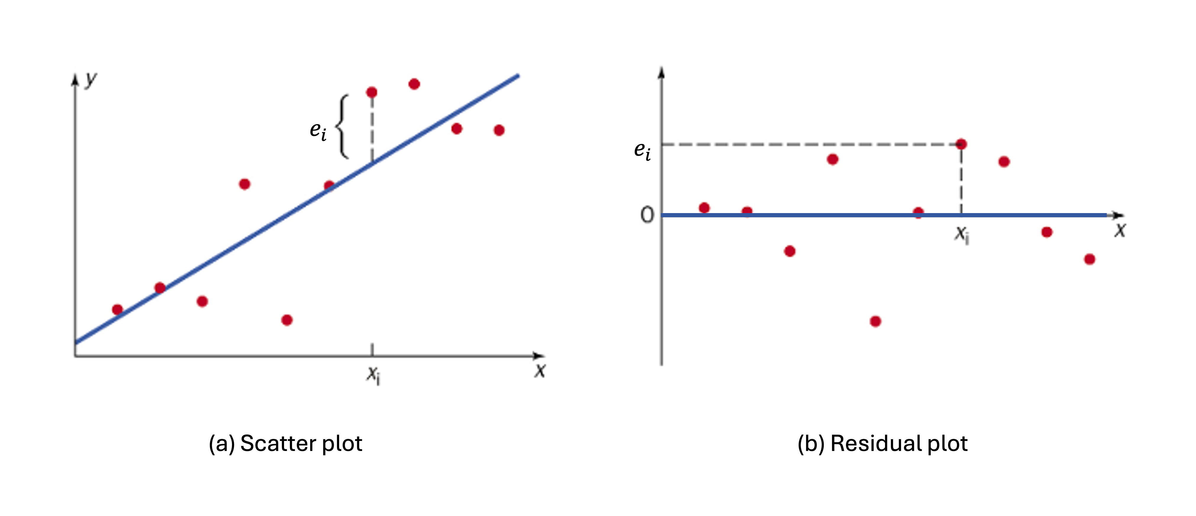
Fig. 13.22 Comparison of scatter plot and residual plot

A residual plot can be viewed as the original scatter plot rotated so that the regression line becomes horizontal. This removes the visual bias of the tilted trend line and highlights the deviations from the fitted line.

Scatter plots and residual plots are typically used together to assess two assumptions: linearity and constant variance.

Characteristics of Ideal Scatter and Residual Plots

When the linearity and constant variance assumptions hold, the points on both the scatter plot and residual plot form a random scatter around their respective summary lines, with a roughly constant spread across the \(x\)-axis.

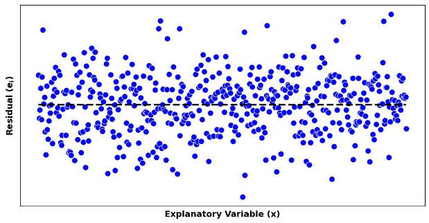
Fig. 13.23 A residual plot showing no signs of assumption violation

Signs of Assumption Violation on Scatter and Resiual Plots

1. Violation of the Linearity Assumption

If residuals systematically fall below the zero line in certain regions of \(x\) values and above the line in others, this suggests the true relationship is non-linear.

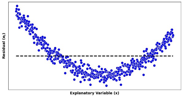
Fig. 13.24 Resiual plots with linearity assumption violated

2. Violation of the Constant Variance Assumption

If the spread of points around the trend line is inconsistent, the data likely violate the constant variance assumption.

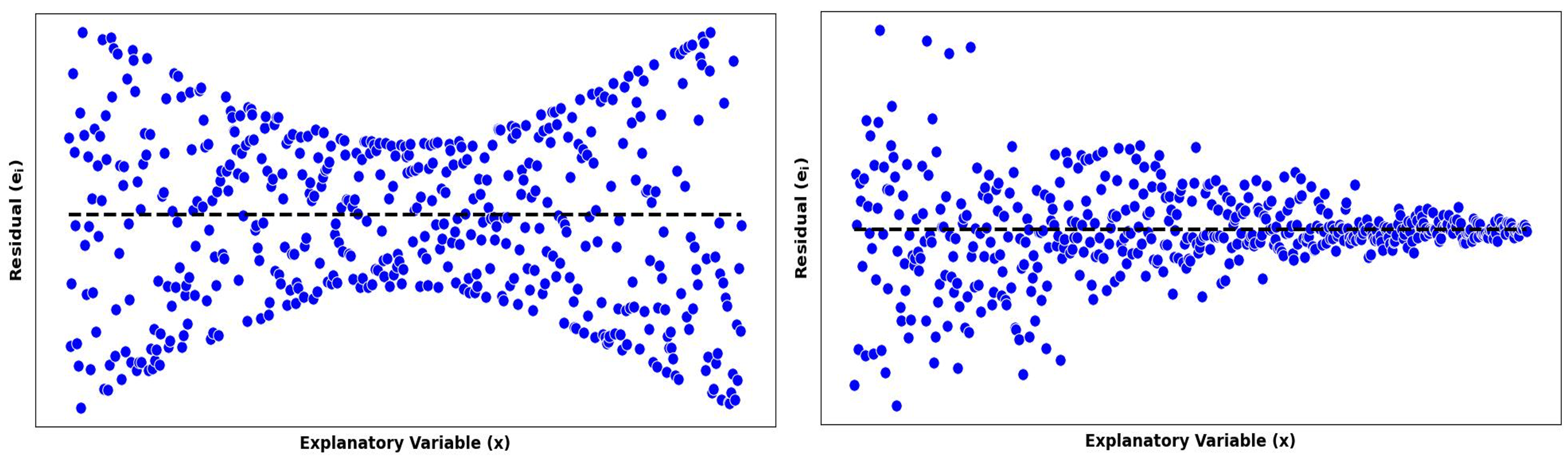
Fig. 13.25 Resiual plots with constant variance assumption violated

• Hourglass Pattern: The spread is larger for extreme values of \(X\) than in the middle range.

• Cone Pattern: As \(X\) increases, the residual errors become larger.

Other patterns of non-constant variance can also occur. Even without systematic patterns, an inconsistent spread alone is a significant sign of assumption violation.

3. Outliers

Recall that scatter plots are also used to identify potential outliers and influential points. Residual plots can serve the same purpose.

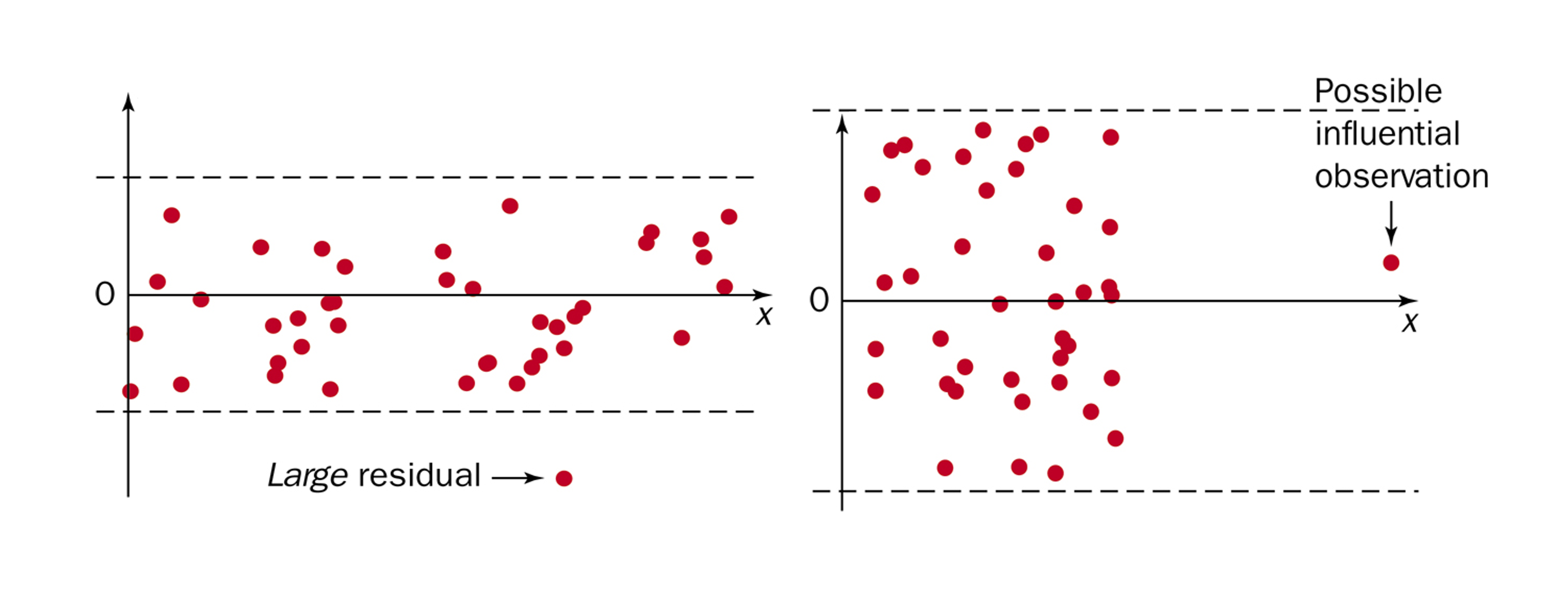
Fig. 13.26 Resiual plots with outliers; left plot shows a \(y\)-outlier, and right shows an \(x\)-outlier that potentially has high influence on the model.

Violations May or May not Occur Simultaneously

While Fig. 13.24 show signs of non-linearity, it does not violate the constant variance assumption since the bandwidth of data points around their true summary curve (quadratic association) is reasonably constant.

Likewise, Fig. 13.25 shows no sign of non-linearity, as the patterns of spread above and below the zero line are roughly symmetric.

Be aware that different types of violations may occur simultaneously or separately, and be prepared to distinguish one case from another on the graphs.

Exercise: draw a residual plot that shows violation of lineary and constant variance assumptions simultaneously.

13.3.3. Histogram and Normal Probability Plot of Residuals for Normality

To verify normality of the error terms, we construct a histogram and a normal probability plot of the residuals.

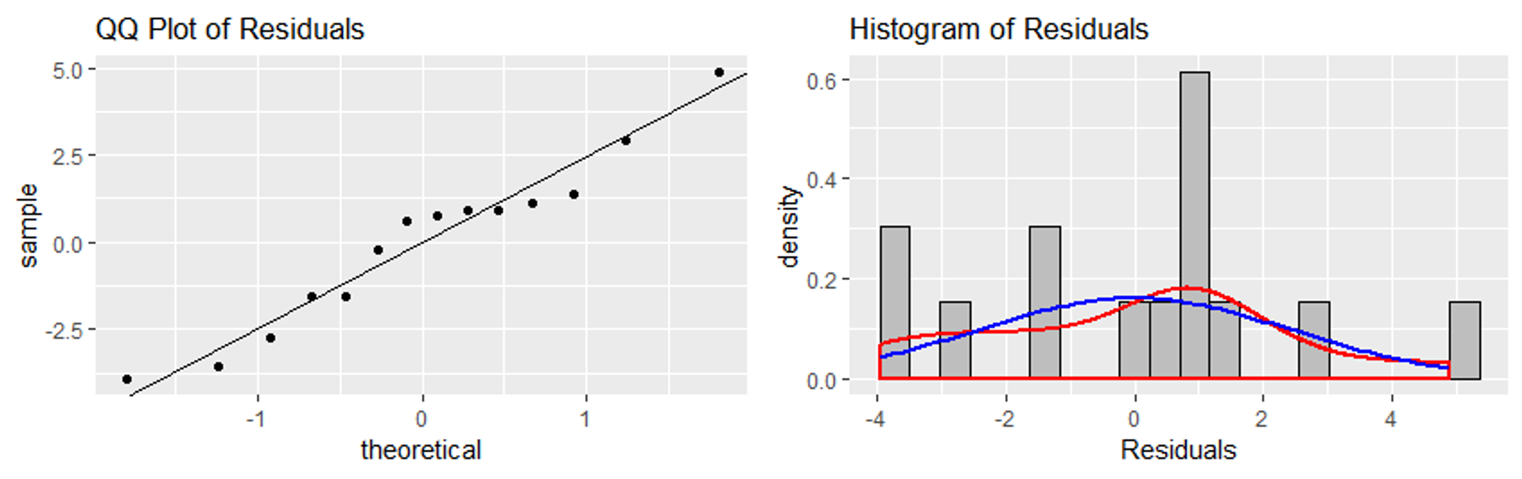
Fig. 13.27 Histogram and normal probability plot of residuals

These plots are used in the same way as in any prior context of normality assessment. We check whether the points follow a straight line on the normal probability plot and whether the histogram is bell-shaped.

13.3.4. Summary of Diagnostic Tools and Comprehensive Eaxmples

We have introduced four graphical tools to assess the assumptions of linear regression. See the table below for a summary:

Assumption	Graphical Tools
SRS	None (must be ensured through experimental design)
Linearity	Scatter plot and residual plot
Constant variance	Scatter plot and residual plot
Normality of errors	Histogram and QQ plot of residuals

Example 💡: Comprehensive Diagnostic Exercise

For each of the following sets of graphical representations, assess whether the data set meets the assumptions required for valid linear regression.

Example 1

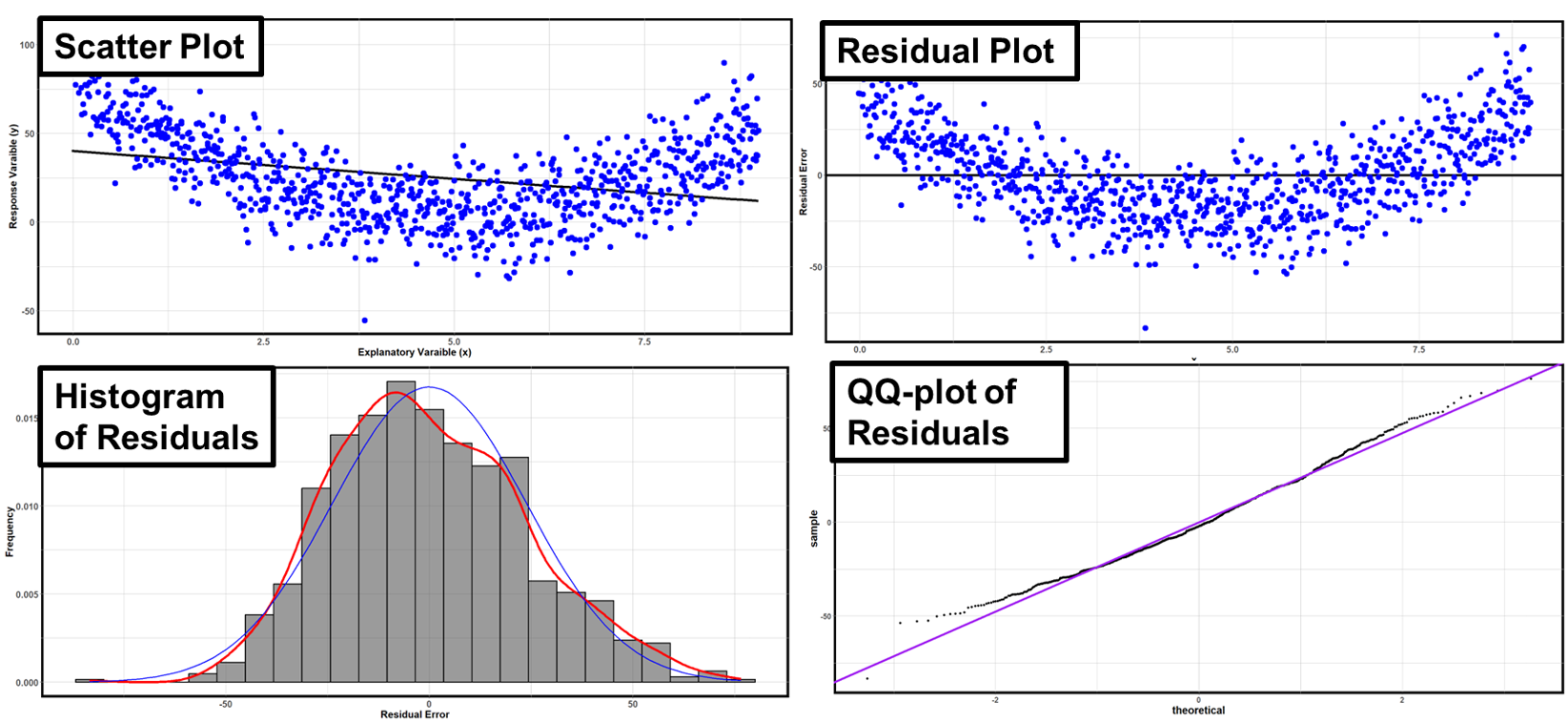
Fig. 13.28 Example 1 of graphical diagnosis

• Scatter plot and residual plot show a systematic curved pattern.

• If the correct summary curve is used (quadratic form), then the size of their vertical spread would not vary by the \(x\)-values. So non-constant variance is not a concern.

• Histogram and normal probability plots look reasonable.

This data set violates the linearity assumption.

Example 2

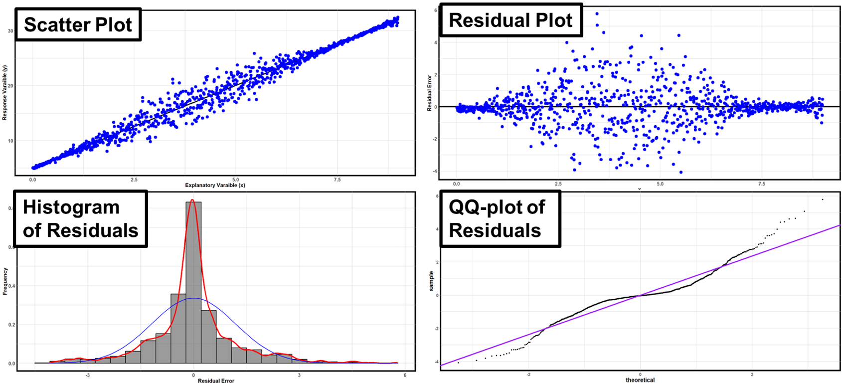
Fig. 13.29 Example 2 of graphical diagnosis

• The dots follow a linear pattern according to both the scatter plot and the residual plot—they form mirror images below and above their summary lines.

• The spread of the points are narrower in the two ends than in the middle region. This raises a concern for non-constant variance.

• The histogram and the QQ plot indicate that the error distribution has heavier tails than the blue curve. The error distribution may not be normal.

This data set violates the constant-variance assumption and is suspected to have non-normal error terms.

When Assumptions Are Violated

If diagnostic procedures reveal serious assumption violations, we should not proceed with linear regression analysis. Instead, we should take an appropriate measure to mitigate the effect of the violation or use a different analysis method.

Linearity Violations:

• Consider transformations of variables (log, square root, etc.)

• Fit non-linear models (beyond course scope)

• Use piecewise or segmented regression for different regions

Constant Variance Violations:

• Variable transformations may help stabilize variance

• Weighted least squares methods (beyond course scope)

• Robust regression techniques

Normality Violations:

• Often less critical for large sample sizes due to Central Limit Theorem

• Bootstrap methods for inference (beyond course scope)

• Non-parametric alternatives

Independence Violations:

• Time series methods for temporally correlated observations

• Mixed effects models for clustered data

---

13.3.5. The F-Test for Model Utility

Once we have verified that our model assumptions are reasonably satisfied, we proceed with statistical inference. The first question we typically ask is: “Does the simple linear regression model provide useful information about the relationship between the explanatory and response variables?”

We organize our answer to this question into the usual four-step hypothesis test. We refer to the ANOVA table constructed in Chapter 13.2.

Step 1: Parameter of Interest

The focus of this test is on the overall usefulness of the linear relationship rather than on specific parameters. Therefore, it is okay to skip explicit parameter definition.

Step 2: Hypotheses

• \(H_0:\) There is no linear association between \(X\) and \(Y\).

• \(H_0:\) There is a linear association between \(X\) and \(Y\).

Important: Always state the hypotheses using the experimental context, replacing “X” and “Y” with the actual variable names and providing sufficient background information.

Step 3: Test Statistic and P-value

Recall that MSR is a scaled measurement of the variability attributed to the model structure, while MSE is a scaled measure of random error. Therefore, if MSR is substantially greater than MSE, we can consider the model to be statistically significant.

The corresponding test statistic is:

\[F_{TS} = \frac{\text{MSR}}{\text{MSE}},\]

with degrees of freedom \(df_1 = 1\) and \(df_2 = n-2\).

A large observed value of \(F_{TS}\) is in favor of the alternative hypothesis that the model is significant. Therefore,

\[\text{p-value} = P(F_{1, n-2} > f_{TS}).\]

Step 4: Decision and Conclusion

• If p-value ≤ \(\alpha\):

  Reject \(H_0\). At the \(\alpha\) significance level, we have sufficient evidence to conclude that there is a linear association between [explanatory variable] and [response variable] in [context].”

• If p-value > \(\alpha\):

  Fail to reject \(H_0\). At the \(\alpha\) significance level, we do not have sufficient evidence to conclude that there is a linear association between [explanatory variable] and [response variable] in [context].”

Example 💡: Blood Pressure Study, Continued

Assuming that the assumptions of linear regression have been verified, perform the \(F\)-test for model utility using \(\alpha = 0.05.\) Use the partially filled ANOVA table from the previous lesson:

Source	df	Sum of Squares	Mean Square	F-statistic	p-value
Regression	1	\(555.7126\)	\(555.7126\)	?	?
Error	\(9\)	\(382.8267\)	\(42.5363\)
Total	\(10\)	\(938.5393\)

Step 1: Parameter Definition

This step is skipped for model utility tests.

Step 2: Hypotheses:

• \(H_0\): There is no linear association between patient age and change in blood pressure.

• \(H_a\): There is a linear association between patient age and change in blood pressure.

Step 3: Computation

\[f_{TS} = \frac{\text{MSR}}{\text{MSE}} = \frac{555.7126}{42.5363} = 13.06\]

The test statistic has two degrees of freedom: \(df_1=1\) and \(df_2=9\). The \(p\)-value is:

\[P(F_{1,9} > 13.06) = 0.0055.\]

Step 4: Conclusion

At \(\alpha = 0.05\), we reject \(H_0\) and conclude that there is sufficient evidence of a linear association between patient age and change in blood pressure.

---

13.3.6. Distributional Properties of the Slope and Intercept Estimators

To develop inference procedures for \(\beta_0\) and \(\beta_1\), we need to understand the statistical properties of their estimators, \(b_0\) and \(b_1\). This draws distinction from our focus on \(b_0\) and \(b_1\) as estimates so far, yielding one set of realized values based on a single data. We would now like to study their behaviors across many different datasets.

1. Slope and Intecept Estimators Are Linear Combinations of the Responses

The first step in constructing inference for regression parameters is to recognize that their estimators are linear combinations of the response variables, \(Y_i, i=1,\cdots, n\). Capital \(Y\) is used throughout this section to emphasize that we are discussing responses as random variables, not their observed values. The values of the explanatory variable are still considered given and fixed.

We first show that the slope estimator \(b_1\) is a linear combination of \(Y_i, i=1,\cdots, n\), starting with its definition:

(13.10)\[\begin{split}b_1 &= \frac{\sum_{i=1}^n x_iY_i - n\bar{x}\bar{Y}}{S_{XX}} \\ &= \frac{\sum_{i=1}^n x_iY_i - \sum_{i=1}^n\bar{x}Y_i}{S_{XX}}\\ &= \sum_{i=1}^n \left(\frac{x_i - \bar{x}}{S_{XX}}\right) Y_i\end{split}\]

Each coefficient to the responses above only consists of non-random quantities involving the explanatory variable.

For the intercept estimator, we borrow the result of Eq. (13.10).

\[\begin{split}b_0 &= \bar{Y} -b_1\bar{x} \\ &= \sum_{i=1}^n \frac{1}{n}Y_i - \bar{x}\sum_{i=1}^n \left(\frac{x_i - \bar{x}}{S_{XX}}\right) Y_i\\ &= \sum_{i=1}^n \left(\frac{1}{n} - \frac{\bar{x}}{S_{XX}}(x_i - \bar{x})\right) Y_i\\\end{split}\]

Again, the coefficient of each term above consists of non-random quantities involving only the sample size and the explanatory values.

‼️ Key Observation

Recall that each \(Y_i\) is normally disributed given an observed \(x_i\). Since both \(b_1\) and \(b_0\) are linear combinations of normal random variables, they must also be normally distributed. We now proceed to state their expectations and variances.

2. The Expectation and Variance of the Parameter Estimators

The Slope Estimator

\[\begin{split}&E[b_1] = \beta_1\\ &\text{Var}(b_1) = \frac{\sigma^2}{S_{XX}}\end{split}\]

The Intercept Estimator

\[\begin{split}&E[b_0] = \beta_0\\ &\text{Var}(b_0) = \sigma^2\left(\frac{1}{n} + \frac{\bar{x}^2}{S_{XX}}\right)\end{split}\]

Key Insights:

• Both \(b_1\) and \(b_0\) are unbiased estimators of \(\beta_1\) and \(\beta_0\), respectively.

• The slope variance depends only on the error variance and the spread of the explanatory values.

• The intercept variance includes additional uncertainty when \(\bar{x} \neq 0\).

Derive the Results as an Independent Exercise

The expectations and variances of both estimators can be derived using general properties and some algebraic manipulation. You are encouraged to verify these results as an independent exercise.

3. The Complete Distribution of the Estimators

Provided that all model assumptions hold,

\[b_1 \sim N\left(\beta_1, \frac{\sigma^2}{S_{XX}}\right)\]

\[b_0 \sim N\left(\beta_0, \sigma^2 \left(\frac{1}{n} + \frac{\bar{x}^2}{S_{XX}}\right)\right)\]

4. Estimated Standard Errors and t-Distribution

Since \(\sigma^2\) is unknown, we replace it with its estimate \(s^2 = MSE\) to obtain the estimated standard errors:

\[\widehat{SE}(b_1) = \sqrt{\frac{MSE}{S_{XX}}}\]

\[\widehat{SE}(b_0) = \sqrt{MSE\left(\frac{1}{n} + \frac{\bar{x}^2}{S_{XX}}\right)}\]

Studentization of each estimator then gives us a \(t\)-distributed random variable, both with \(df=n-2\):

\[\frac{b_1 - \beta_1}{\widehat{SE}(b_1)} \sim t_{n-2}\]

\[\frac{b_0 - \beta_0}{\widehat{SE}(b_0)} \sim t_{n-2}\]

We use these as the foundation for confidence regions and hypothesis tests on the true values of the regression parameters, \(\beta_1\) and \(\beta_0\).

13.3.7. Confidence Regions for Parameters

Recall the general form of a \(t\)-confidence region:

\[\text{estimate} \pm t_{crit} \widehat{SE}(\text{estimate})\]

The table below applies the general form to all possible parameter-side combination:

Side	\(\beta_0\)	\(\beta_1\)
CI	\[b_0 \pm t_{\alpha/2, n-2}\sqrt{MSE\left(\frac{1}{n} + \frac{\bar{x}^2}{S_{XX}}\right)}\]	\[b_1 \pm t_{\alpha/2, n-2} \sqrt{\frac{MSE}{S_{XX}}}\]
UCB	\[b_0 + t_{\alpha, n-2}\sqrt{MSE\left(\frac{1}{n} + \frac{\bar{x}^2}{S_{XX}}\right)}\]	\[b_1 + t_{\alpha, n-2} \sqrt{\frac{MSE}{S_{XX}}}\]
LCB	\[b_0 - t_{\alpha, n-2}\sqrt{MSE\left(\frac{1}{n} + \frac{\bar{x}^2}{S_{XX}}\right)}\]	\[b_1 - t_{\alpha, n-2} \sqrt{\frac{MSE}{S_{XX}}}\]

13.3.8. Hypothesis Testing for the Slope Parameter

Step 1: Parameter of Interest

Define \(\beta_1\) as the slope of the true regression line relating [explanatory variable] to [response variable]. Make sure to use experiment-specific variable names and context.

Step 2: Hypotheses

It is possible to construct a one-sided or two-sided hypothesis test for the slope parameter against any null value \(\beta_{10}\).

\[\begin{split}&H_0: \beta_{1} (=, \leq, \geq) \beta_{10}\\ &H_1: \beta_{1} (\neq, >, <) \beta_{10}\end{split}\]

The most common hypothesis is the two-sided variant with the null value \(\beta_{10} = 0\).

\[\begin{split}&H_0: \beta_1 = 0\\ &H_a: \beta_1 \neq 0\end{split}\]

Step 3: Test Statistic and P-value

\[T_{ts} = \frac{b_1 - \beta_{10}}{\widehat{SE}(b_1)}\]

has \(t\)-distribution with \(df = n-2\). Once an observed value \(t_{TS}\) is obtained, the \(p\)-value computation should align with the sidedness of the hypothesis.

• Two-sided: \(p\)-value \(= 2P(T_{n-2} > |t_{TS}|)\)

• Upper-tailed: \(p\)-value \(= P(T_{n-2} > t_{TS})\)

• Lower-tailed: \(p\)-value \(= P(T_{n-2} < t_{TS})\)

Step 4: Decision and Conclusion

Compare p-value to \(\alpha\) and draw conclusions about the slope parameter in context.

Hypothesis Tests for the Intercept

Hypothesis tests on \(\beta_0\) can be constructed in a similar manner. They are not explored in detail because:

1. The procedure only differs by the form of the standard error estimate, and

2. The intercept often does not have any practial significance.

Example 💡: Blood Pressure Study, Continued

For the blood pressure vs age data set, perform a hypothesis test to determine if the slope parameter is non-zero. Then, construct a corresponding confidence region.

Step 1: Define the parameter of interest

We are interested in \(\beta_1\), the true change in blood pressure per year increase in patient age.

Step 2: State the hypotheses

\[\begin{split}&H_0: \beta_1 = 0\\ &H_a: \beta_1 \neq 0\end{split}\]

Step 3: Computation

The test statistic is:

\[t_{TS} = \frac{b_1-0}{\sqrt{\text{MSE}/S_{xx}}}\frac{-0.526 - 0}{0.146} = -3.61.\]

The \(p\)-value is:

\[2P(T_9 > 3.61) = 0.0055.\]

Step 4: Conclusion

\(p\)-value \(=0.0055 < \alpha\). The null hypothesis is rejected. At \(\alpha=0.05\), there is enough evidence to conclude that the slope of the true linear association between age and change in blood pressure is different than \(0\).

95% Confidence Interval:

The confidence region corresponding to a two-sided hypothesis test is a confidence interval. Use R to compute the critical value:

qt(0.025, df=9, lower.tail=FALSE)
#2.262

Then putting the components together,

\[-0.526 \pm (2.262)(0.146) = -0.526 \pm 0.330 = (-0.856, -0.196).\]

We are 95% confident that each additional year of age is associated with a decrease in blood pressure between 0.196 and 0.856 mm Hg after treatment.

13.3.9. Special Case: Equivalence of F-test and t-test

For simple linear regresssion, the hypothesis test on \(H_a: \beta_1 \neq 0\) is equivalent to the \(F\)-test for model utility. Intuitively, this makes sense because, in order for the model to meaningfully describe the response variable, the explanatory variable must have a significant association with it.

Mathematically, this equivalence is explained through the special equality:

\[T_{ts}^2 = F_{TS}\]

To see why this is true, recall that \(b_1 = \frac{S_{XY}}{S_{XX}}\) and \(\text{MSR} = b_1\text{S}_{XY}\). Using these,

\[T_{ts}^2 = \frac{b_1^2}{\text{MSE}/S_{XX}} = \frac{b_1 \frac{S_{XY}}{S_{XX}} S_{XX}}{MSE} = \frac{MSR}{MSE}\]

This implies that both tests provide identical p-values and conclusions.

The Equivalence Only Holds for Simple LR

The two tests serve different purposes in general linear regression with multiple predictors:

• The \(F\)-test assesses whether at least one of the predictors provide useful information about the response variable.

• The \(t\)-test on a slope parameter assesses whether the single corresponding predictor is useful.

Example 💡: Blood Pressure Study, Continued

For the blood pressure dataset, verify the equivalence of the model utility \(F\)-test and the two-tailed \(t\)-test on the slope parameter against \(\beta_{10}=0\).

From the two previous examples,

• \(t_{TS}^2 = (-3.61)^2 = 13.03\)

• \(f_{TS}=13.06\)

• There is a small difference due to rounding, but both tests give \(p\)-value \(= 0.0055\). ✔

13.3.10. Bring It All Tgether

Key Takeaways 📝

1. Diagnostic plots are essential for verifying model assumptions before conducting hypothesis tests or constructing confidence intervals.

2. Four key diagnostic tools work together: scatter plots, residual plots, histograms of residuals, and QQ plots provide complementary information about different aspects of model adequacy.

3. The model utility F-test assesses whether the linear relationship explains a significant portion of the variability in the response variable.

4. Inference on the slope and intercept adapts familiar principles used in previous inference procedures on single parameters.

6. In simple linear regression, the model utility F-test is equivalent to the \(t\)-test on \(H_a: \beta_1 \neq 0\).

13.3.11. Exercises

Exercise 1: Diagnostic Plot Interpretation

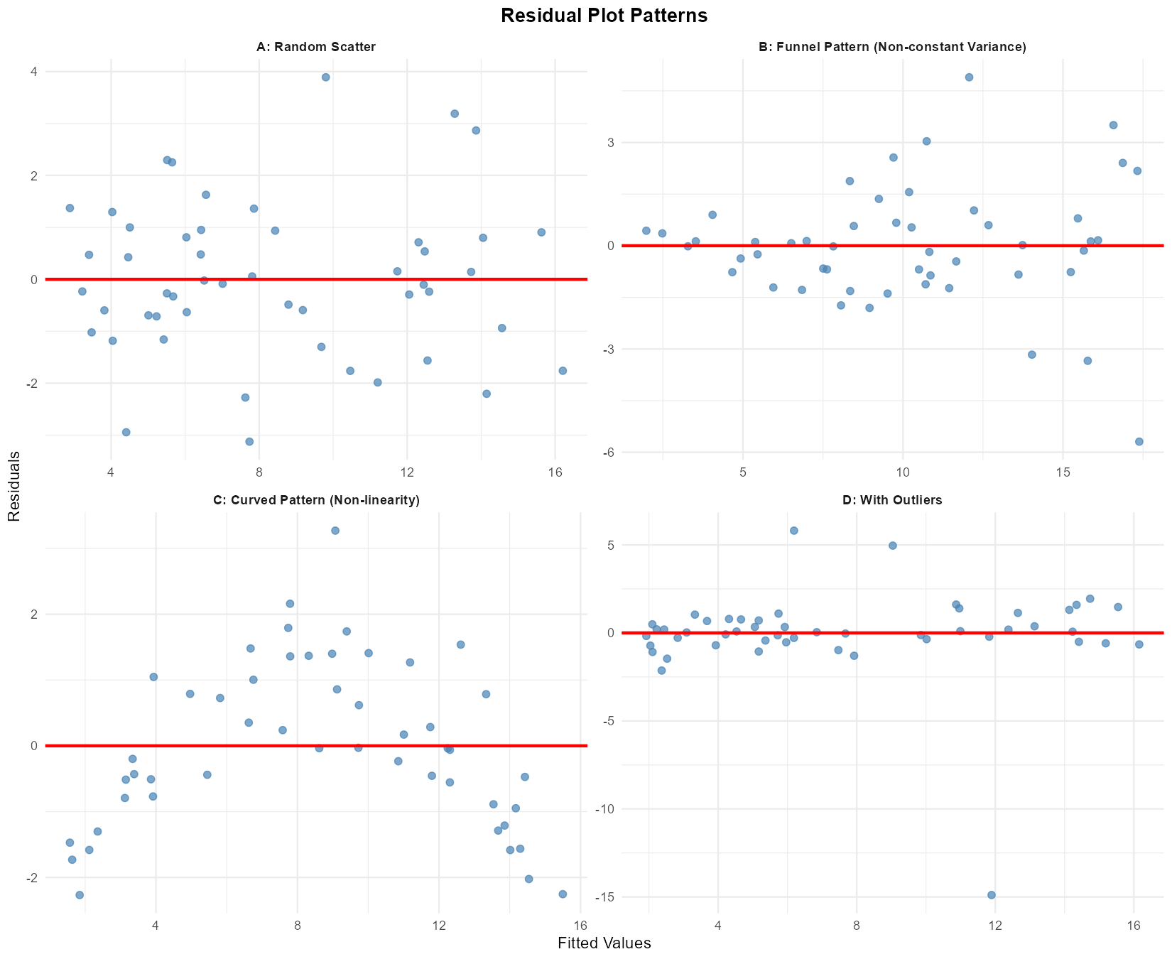
Fig. 13.30 Four residual plots showing different patterns

For each residual plot above (A, B, C, D), identify:

1. Whether the linearity assumption appears satisfied

2. Whether the constant variance (homoscedasticity) assumption appears satisfied

3. Any outliers or influential points

4. Overall assessment: Is the linear regression model appropriate?

Solution

Plot	Linearity	Constant Var	Outliers	Model Appropriate?
A	✓ Satisfied	✓ Satisfied	None	Yes - proceed
B	✓ Satisfied	✗ Funnel pattern	None	No - variance issue
C	✗ Curved	✓ Satisfied	None	No - linearity violated
D	✓ Satisfied	✓ Satisfied	Yes (3)	Caution - investigate

---

Exercise 2: Complete Diagnostic Analysis

A software engineer models the relationship between lines of code (X, in thousands) and execution time (Y, in seconds) for \(n = 25\) programs.

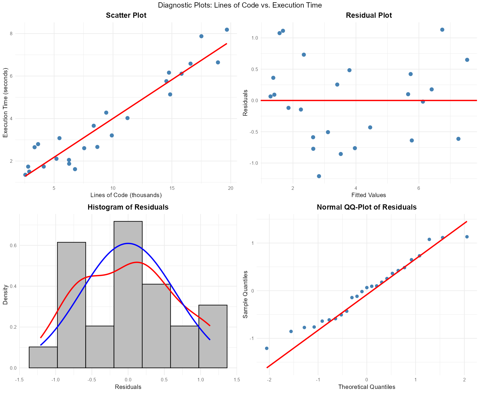
Fig. 13.31 Diagnostic plots: scatter plot, residual plot, histogram, and QQ-plot

Based on the four diagnostic plots:

1. Assess the linearity assumption using the scatter plot and residual plot.

2. Assess the constant variance assumption using the residual plot.

3. Assess the normality assumption using the histogram and QQ-plot.

4. Are there any apparent outliers? If so, describe them.

5. Would you proceed with inference based on this model? Justify your answer.

Solution

Part (a): Linearity assessment

• Scatter plot: Shows a clear positive linear trend with points following an approximately straight pattern

• Residual plot: Residuals appear randomly scattered around zero with no systematic curvature

Conclusion: Linearity assumption is satisfied ✓

Part (b): Constant variance assessment

• Residual plot: The vertical spread of residuals appears roughly constant across all fitted values

• No funnel shape or systematic change in spread

Conclusion: Equal variance assumption is satisfied ✓

Part (c): Normality assessment

• Histogram: Residuals show an approximately symmetric, bell-shaped distribution

• The kernel density (red) and normal curve (blue) align reasonably well

• QQ-plot: Points fall close to the reference line with no major systematic departures

Conclusion: Normality assumption is satisfied ✓

Part (d): Outliers

No obvious outliers. All points appear consistent with the general pattern, and no residuals are extremely far from zero.

Part (e): Proceed with inference?

Yes, inference is appropriate. All four assumptions (LINE) appear to be satisfied:

• Linearity: Yes (scatter and residual plots)

• Independence: Assumed (no time ordering mentioned)

• Normality: Yes (histogram and QQ-plot)

• Equal variance: Yes (residual plot)

The model is well-suited for hypothesis tests and confidence intervals.

---

Exercise 3: ANOVA F-Test for Model Utility

An industrial engineer studies the relationship between conveyor belt speed (ft/min) and defect rate (defects per 1000 units). With \(n = 18\) production runs:

• SSR = 245.6

• SSE = 89.4

1. State the hypotheses for testing model utility.

2. Complete the ANOVA table and calculate the F-statistic.

3. Find the p-value using R: pf(F_stat, 1, 16, lower.tail = FALSE)

4. At \(\alpha = 0.05\), what is your conclusion? State it in context using proper conclusion format.

Solution

Part (a): Hypotheses

• \(H_0: \beta_1 = 0\) (There is no linear relationship between conveyor speed and defect rate)

• \(H_a: \beta_1 \neq 0\) (There is a linear relationship between conveyor speed and defect rate)

Part (b): ANOVA Table

Source	df	SS	MS	F
Regression	1	245.6	245.6	43.97
Error	16	89.4	5.5875
Total	17	335.0

Calculations:

• \(df_{Error} = n - 2 = 18 - 2 = 16\)

• \(MSR = 245.6/1 = 245.6\)

• \(MSE = 89.4/16 = 5.5875\)

• \(F = MSR/MSE = 245.6/5.5875 = 43.97\)

Part (c): P-value

pf(43.97, 1, 16, lower.tail = FALSE)
# p-value = 6.86e-06

Part (d): Conclusion

At \(\alpha = 0.05\), since p-value (6.86 × 10⁻⁶) < 0.05, we reject \(H_0\).

There is sufficient evidence to conclude that there is a significant linear relationship between conveyor belt speed and defect rate.

---

Exercise 4: Inference for the Slope

From a regression of drug dosage (mg) on patient recovery time (days) with \(n = 24\) patients:

• \(b_1 = -0.85\) (days per mg)

• \(SE_{b_1} = 0.23\)

1. Construct a 95% confidence interval for the true slope \(\beta_1\).

2. Interpret this confidence interval in context.

3. Test \(H_0: \beta_1 = 0\) vs \(H_a: \beta_1 \neq 0\) at \(\alpha = 0.05\).

   • State the test statistic formula and calculate \(t_{TS}\)

   • Find the p-value

   • State your conclusion in context using proper format

4. Is the result of part (c) consistent with your confidence interval in part (a)? Explain.

Solution

Part (a): 95% CI for slope

Degrees of freedom: \(df = n - 2 = 24 - 2 = 22\)

Critical value: \(t_{0.025, 22} = 2.074\)

\[CI = b_1 \pm t^* \cdot SE_{b_1} = -0.85 \pm 2.074(0.23) = -0.85 \pm 0.477\]

95% CI: (−1.33, −0.37)

Part (b): Interpretation

We are 95% confident that the true slope \(\beta_1\) is between −1.33 and −0.37 days per mg.

In context: For each additional mg of drug dosage, recovery time decreases by between 0.37 and 1.33 days, on average.

Part (c): Hypothesis test

Step 1: Parameter: \(\beta_1\) = true change in recovery time per mg increase in dosage

Step 2: \(H_0: \beta_1 = 0\) vs. \(H_a: \beta_1 \neq 0\)

Step 3: Test statistic:

\[t_{TS} = \frac{b_1 - 0}{SE_{b_1}} = \frac{-0.85}{0.23} = -3.70\]

P-value (two-sided): 2 * pt(abs(-3.70), 22, lower.tail = FALSE) = 0.0012

Step 4: At \(\alpha = 0.05\), since p-value (0.0012) < 0.05, we reject \(H_0\).

There is sufficient evidence to conclude that drug dosage has a significant linear effect on recovery time.

Part (d): Consistency

Yes, the results are consistent. The CI (−1.33, −0.37) does not contain 0, which corresponds to rejecting \(H_0: \beta_1 = 0\). This illustrates the duality between confidence intervals and hypothesis tests.

---

Exercise 5: Inference for the Intercept

Using the drug dosage regression from Exercise 4:

• \(b_0 = 14.2\) (days)

• \(SE_{b_0} = 1.85\)

• \(n = 24\)

1. Interpret \(b_0\) in context. Is this interpretation meaningful?

2. Construct a 90% confidence interval for \(\beta_0\).

3. Test \(H_0: \beta_0 = 12\) vs \(H_a: \beta_0 \neq 12\) at \(\alpha = 0.10\).

Solution

Part (a): Interpretation of b₀

\(b_0 = 14.2\) represents the predicted recovery time (in days) when drug dosage is 0 mg.

Is it meaningful? Only if dosage = 0 is within or near the range of observed data. If the study only included positive dosages (e.g., 5-50 mg), then \(b_0\) is an extrapolation and may not have practical meaning. It would represent the baseline recovery time without the drug.

Part (b): 90% CI for β₀

\(df = 22\), \(t_{0.05, 22} = 1.717\)

\[CI = 14.2 \pm 1.717(1.85) = 14.2 \pm 3.18\]

90% CI: (11.02, 17.38)

Part (c): Test H₀: β₀ = 12

Test statistic:

\[t_{TS} = \frac{b_0 - 12}{SE_{b_0}} = \frac{14.2 - 12}{1.85} = \frac{2.2}{1.85} = 1.19\]

P-value: 2 * pt(1.19, 22, lower.tail = FALSE) = 0.247

At \(\alpha = 0.10\), since p-value (0.247) > 0.10, we fail to reject \(H_0\).

There is not sufficient evidence to conclude that the true intercept differs from 12 days.

---

Exercise 6: F-test and t-test Relationship

For a simple linear regression with \(n = 30\) observations, the following results were obtained:

• t-statistic for testing \(H_0: \beta_1 = 0\): \(t_{TS} = 4.28\)

• F-statistic for model utility: \(F_{TS} = 18.32\)

1. Verify that \(F_{TS} = t_{TS}^2\) (allowing for rounding).

2. What are the degrees of freedom for the t-test? For the F-test?

3. Why is this relationship only true for simple linear regression (one predictor)?

4. Using pt() and pf(), verify that the p-values are the same.

Solution

Part (a): Verify F = t²

\(t_{TS}^2 = (4.28)^2 = 18.32 = F_{TS}\) ✓

The relationship holds exactly.

Part (b): Degrees of freedom

• t-test: \(df = n - 2 = 30 - 2 = 28\)

• F-test: \(df_1 = 1\) (numerator), \(df_2 = n - 2 = 28\) (denominator)

Part (c): Why only for simple linear regression?

This relationship \(F = t^2\) holds only when:

1. There is exactly one predictor (df₁ = 1 for the F-test)

2. The t-test is for \(H_0: \beta_1 = 0\)

In multiple regression with \(k > 1\) predictors, the overall F-test has \(df_1 = k\), and there’s no single t-statistic that corresponds to it. Each predictor has its own t-test, but these are not equivalent to the overall F-test.

Part (d): P-value verification

# t-test p-value (two-sided)
2 * pt(4.28, 28, lower.tail = FALSE)
# [1] 0.000196

# F-test p-value
pf(18.32, 1, 28, lower.tail = FALSE)
# [1] 0.000196

The p-values are identical (within rounding), confirming the equivalence of the two tests for simple linear regression.

---

Exercise 7: Comprehensive Hypothesis Test

A civil engineer studies the relationship between traffic volume (vehicles per hour) and road surface wear (mm of depth reduction per year). Data from \(n = 15\) road sections yields:

• \(\hat{y} = 0.12 + 0.0008x\)

• \(R^2 = 0.72\)

• \(MSE = 0.0045\)

• \(S_{XX} = 125000000\)

1. Calculate \(SE_{b_1}\).

2. Test whether there is a significant positive relationship between traffic volume and road wear at \(\alpha = 0.01\).

   Step 1: Define the parameter of interest.

   Step 2: State \(H_0\) and \(H_a\) (in symbols and words).

   Step 3: Calculate the test statistic and p-value. Report degrees of freedom.

   Step 4: State your conclusion in context.

3. Construct a 99% confidence interval for \(\beta_1\).

4. Construct a 99% lower confidence bound for \(\beta_1\).

Solution

Part (a): Calculate SE_b₁

\[SE_{b_1} = \sqrt{\frac{MSE}{S_{XX}}} = \sqrt{\frac{0.0045}{125000000}} = \sqrt{3.6 \times 10^{-11}} = 1.90 \times 10^{-5}\]

Part (b): Four-Step Hypothesis Test

Step 1: Let \(\beta_1\) = the true change in road wear (mm/year) per additional vehicle per hour.

Step 2:

• \(H_0: \beta_1 = 0\) (no linear relationship between traffic volume and road wear)

• \(H_a: \beta_1 > 0\) (positive linear relationship — more traffic causes more wear)

Step 3: Test statistic and p-value

\[t_{TS} = \frac{b_1 - 0}{SE_{b_1}} = \frac{0.0008}{1.90 \times 10^{-5}} = 42.1\]

\(df = n - 2 = 13\)

P-value: pt(42.1, 13, lower.tail = FALSE) ≈ 0 (essentially zero)

Step 4: At \(\alpha = 0.01\), since p-value ≈ 0 < 0.01, we reject \(H_0\).

There is sufficient evidence to conclude that there is a significant positive linear relationship between traffic volume and road surface wear.

Part (c): 99% CI for β₁

\(t_{0.005, 13} = 3.012\)

\[CI = 0.0008 \pm 3.012(1.90 \times 10^{-5}) = 0.0008 \pm 0.0000572\]

99% CI: (0.000743, 0.000857)

Part (d): 99% Lower Confidence Bound

For a one-sided bound: \(t_{0.01, 13} = 2.650\)

\[LCB = b_1 - t_{0.01, 13} \cdot SE_{b_1} = 0.0008 - 2.650(1.90 \times 10^{-5}) = 0.000750\]

99% LCB: 0.000750

We are 99% confident that each additional vehicle per hour increases road wear by at least 0.00075 mm/year.

---

Exercise 8: Model Utility with R Output

The following R output is from a regression of patient systolic blood pressure (mmHg) on age (years):

Call:
lm(formula = BP ~ Age, data = patients)

Residuals:
    Min      1Q  Median      3Q     Max
-15.234  -5.891  -0.456   4.789  18.234

Coefficients:
            Estimate Std. Error t value Pr(>|t|)
(Intercept)  95.4500     5.2340  18.236  < 2e-16 ***
Age           0.8920     0.1120   7.964 2.34e-09 ***

Residual standard error: 8.456 on 38 degrees of freedom
Multiple R-squared:  0.6253, Adjusted R-squared:  0.6154
F-statistic: 63.43 on 1 and 38 DF,  p-value: 2.341e-09

1. Write the fitted regression equation.

2. Interpret the slope in context.

3. What is the estimate of \(\sigma\)?

4. What is \(R^2\)? Interpret it.

5. Is the model statistically significant at \(\alpha = 0.01\)? Cite the relevant test statistic and p-value.

6. Construct a 95% confidence interval for the slope using the output.

Solution

Part (a): Fitted equation

\(\widehat{BP} = 95.45 + 0.892 \times Age\)

Or: Predicted Systolic BP = 95.45 + 0.892(Age)

Part (b): Slope interpretation

For each additional year of age, systolic blood pressure increases by an estimated 0.892 mmHg, on average.

Part (c): Estimate of σ

\(\hat{\sigma} = 8.456\) mmHg (residual standard error from output)

Part (d): R² interpretation

\(R^2 = 0.6253\)

Approximately 62.5% of the variation in systolic blood pressure is explained by the linear relationship with age.

Part (e): Model significance

Yes, the model is statistically significant at \(\alpha = 0.01\).

• F-statistic = 63.43 on 1 and 38 DF

• p-value = 2.341 × 10⁻⁹ < 0.01

(Equivalently: t = 7.964 for the slope, p-value = 2.34 × 10⁻⁹)

Part (f): 95% CI for slope

\(t_{0.025, 38} = 2.024\)

\[CI = 0.892 \pm 2.024(0.112) = 0.892 \pm 0.227\]

95% CI: (0.665, 1.119)

We are 95% confident that for each additional year of age, systolic BP increases by between 0.67 and 1.12 mmHg.

---

Exercise 9: Assumption Checking in R

A researcher has fitted a regression model and needs to check assumptions. Complete the following R code to create proper diagnostic plots:

# Fit the model
fit <- lm(y ~ x, data = mydata)

# Create residual plot
mydata$fitted <- ____________
mydata$residuals <- ____________

ggplot(mydata, aes(x = fitted, y = residuals)) +
  geom_point() +
  geom_hline(yintercept = ____, color = "blue", linewidth = 1) +
  labs(title = "Residual Plot",
       x = "____________",
       y = "____________") +
  theme_minimal()

# Create QQ-plot of residuals
ggplot(mydata, aes(sample = ____________)) +
  stat_qq() +
  stat_qq_line(color = "red", linewidth = 1) +
  labs(title = "Normal QQ-Plot of Residuals",
       x = "Theoretical Quantiles",
       y = "Sample Quantiles") +
  theme_minimal()

1. Fill in the blanks to complete the code.

2. What pattern in the residual plot would indicate non-constant variance?

3. What pattern in the QQ-plot would indicate heavy-tailed residuals?

Solution

Part (a): Completed code

# Fit the model
fit <- lm(y ~ x, data = mydata)

# Create residual plot
mydata$fitted <- fitted(fit)
mydata$residuals <- residuals(fit)

ggplot(mydata, aes(x = fitted, y = residuals)) +
  geom_point() +
  geom_hline(yintercept = 0, color = "blue", linewidth = 1) +
  labs(title = "Residual Plot",
       x = "Fitted Values",
       y = "Residuals") +
  theme_minimal()

# Create QQ-plot of residuals
ggplot(mydata, aes(sample = residuals)) +
  stat_qq() +
  stat_qq_line(color = "red", linewidth = 1) +
  labs(title = "Normal QQ-Plot of Residuals",
       x = "Theoretical Quantiles",
       y = "Sample Quantiles") +
  theme_minimal()

Part (b): Non-constant variance pattern

A funnel shape (or megaphone/cone pattern) in the residual plot indicates non-constant variance:

• Opening funnel: Variance increases with fitted values (common)

• Closing funnel: Variance decreases with fitted values (less common)

The vertical spread of residuals should be roughly constant across all fitted values for the assumption to be satisfied.

Part (c): Heavy-tailed residuals

In the QQ-plot, heavy-tailed residuals show an S-shape:

• Points curve below the reference line on the left side

• Points curve above the reference line on the right side

This indicates more extreme values than a normal distribution would produce.

---

13.3.12. Additional Practice Problems

Quick Calculations

1. Given \(b_1 = 3.2\), \(SE_{b_1} = 0.8\), \(n = 22\). Calculate the t-statistic for \(H_0: \beta_1 = 0\).

2. With \(t_{TS} = 2.5\) and \(df = 20\), is the result significant at \(\alpha = 0.05\) (two-sided)?

3. If \(F = 16\) for the model utility test, what is \(|t|\) for the slope test?

True/False

4. If the 95% CI for \(\beta_1\) contains 0, the F-test will not reject \(H_0\).

5. The F-test and t-test for the slope always give identical conclusions in simple linear regression.

6. A significant p-value guarantees the model assumptions are satisfied.

Answers to Practice Problems

Quick Calculations:

1. \(t_{TS} = \frac{b_1 - 0}{SE_{b_1}} = \frac{3.2}{0.8} = 4.0\)

2. Critical value: \(t_{0.025, 20} = 2.086\). Since \(|2.5| > 2.086\), yes, significant at \(\alpha = 0.05\).

3. \(|t| = \sqrt{F} = \sqrt{16} = 4\)

True/False:

4. TRUE — Due to the duality between CIs and hypothesis tests. If 0 is in the CI, the test doesn’t reject \(H_0: \beta_1 = 0\), which is equivalent to the F-test in SLR.

5. TRUE — For simple linear regression, \(F = t^2\) and the p-values are identical.

6. FALSE — A significant p-value only means we reject \(H_0\). Model assumptions must be verified separately through diagnostic plots, not hypothesis tests.