Slides 📊

Download Chapter 4 slides (PPTX)

4.3. Conditional Probability

With the foundations of probability established, we can now extend our toolset to explore how events influence each other. In real-world scenarios, we often have partial information about an experiment’s outcome, and need to update our probability assessments as more information is gathered. Conditional probability provides the mathematical framework for incorporating this new information and analyzing relationships between events.

Road Map 🧭

• Define conditional probability and understand its interpretation.

• Derive the conditional probability formula and the general multiplication rule.

• Understand how tree diagrams represent conditional probabilities graphically.

4.3.1. Understanding Conditional Probability

Conditional probability addresses how the probability of one event changes when we know that another event occurs. It represents the revised probability assessment for an event based on new information.

For example, suppose an AI model is built to detect wolves in an image. If it also received input that the image contains large carnivores, then it would assign a higher probability to the presence of wolves than without this prior information. This additional information changes, or conditions, the probability assessment.

Definition and Notation

The conditional probability of event \(A\) given that event \(B\) occurs is denoted by \(P(A|B)\), read as “the probability of \(A\) given \(B\).”

The conditional probability is computed as

\[P(A|B) = \frac{P(A \cap B)}{P(B)}.\]

This formula is valid only when \(P(B) > 0\); we cannot condition on impossible events, and we cannot divided by \(0\) to obtain a valid probability.

What is happening in the conditional probability formula?

A probability, whether conditional or not, represents the relative size of a part out of a whole.

In non-conditional situations, the relative size of event A is assessed out of the whole sample space.

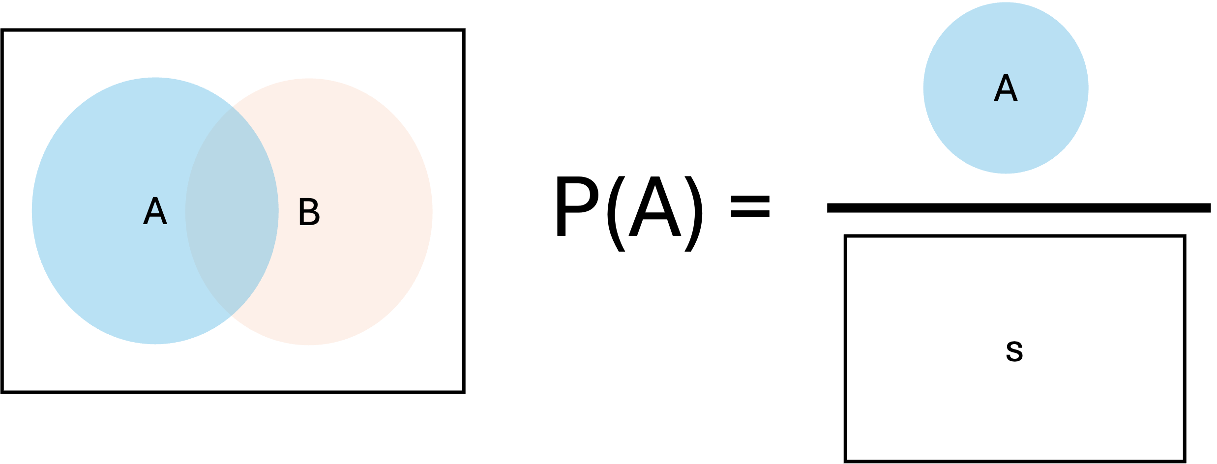
Fig. 4.11 Non-conditional probability

However, by knowing that event \(B\) occurs, our sample space becomes restricted to only the outcomes in \(B\) —anything that does not belong to \(B\) is not a possibility anymore. Within this reduced sample space, we’re interested in the relative size of the regoin which still belongs to event \(A\).

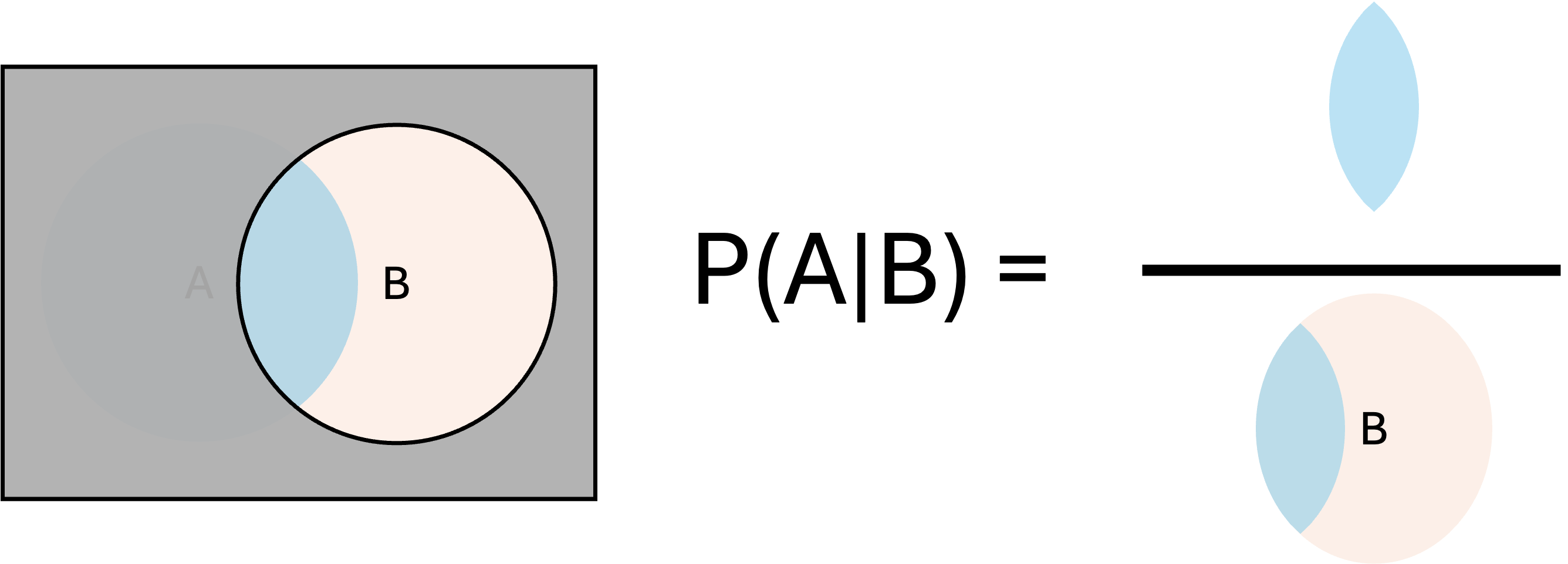
Fig. 4.12 Conditional probability

The numerator of Fig. 4.12 is the Venn diagram representation of \(P(A \cap B)\) and the denominator of \(P(B)\). This graphical expression agrees precisely with the mathematical formula of conditional probability.

Example 💡: Cards from a Deck

Suppse we are drawing a card from a standard deck, where each of the 52 cards has an equal chance of being drawn. Define \(H\) as the event of drawing a heart and \(Q\) as the event of drawing a queen.

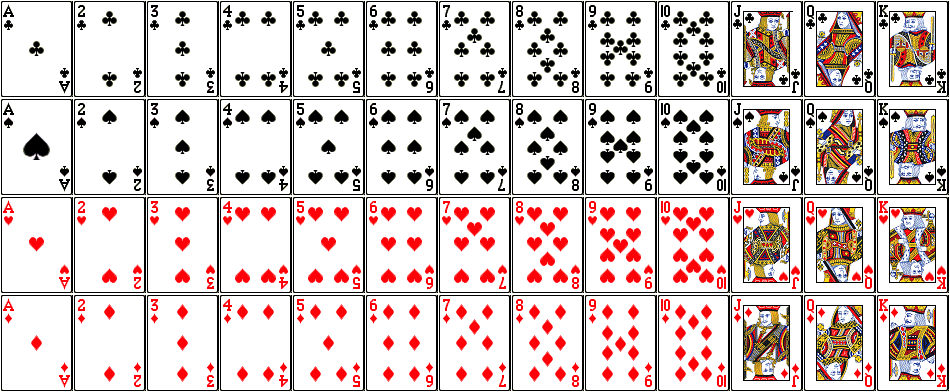
Fig. 4.13 A standard 52-card deck

1. A card has been drawn. If it is known that the card is a heart, what is the probability that it is a queen?

   • \(P(Q ∩ H) = 1/52\) (only one card is both a queen and a heart)

   • \(P(H) = 13/52 = 1/4\) (there are thirteen hearts)

   \[P(Q|H) = \frac{P(Q ∩ H)}{P(H)} = \frac{1/52}{13/52} = \frac{1}{13}.\]

2. If it is known that the card is a queen, what is the probability that it is a heart?

   \(P(Q) = 4/52 = 1/13\) (there are four queens). Therefore,

   \[P(H|Q) = \frac{P(Q ∩ H)}{P(Q)} = \frac{1/52}{1/13} = \frac{1}{4}.\]

🛑 In this example, we computed three closely related two-event probabilities— \(P(Q \cap H), P(Q|H),\) and \(P(H|Q)\)— which yielded different numerical values. It is an important skill to identify which probability a word problem is asking for and then apply the correct formula.

4.3.2. The General Multiplication Rule

The conditional probability formula can be rearranged to give us the general multiplication rule:

\[P(A \cap B) = P(A|B) P(B)\]

This is obtained simply by mupltiplying \(P(B)\) on both sides of the conditional probability formula. This rule allows us to find the probability of the intersection of two events when we know a conditional probability and an unconditional probability.

The formula can also be written as:

\[P(A \cap B) = P(B|A) P(A)\]

Both forms are valid, and which one to use depends on what information is available in a problem.

Extending the General Multiplication Rule to Multiple Events

1. Begin by taking an unconditioned probability of any one event.

2. Multiply the probability of a new event conditional on the event used for step 1.

3. Multiply the probability of another new event conditional on the intersection of all previously used events.

4. Continue in a similar manner.

The order of events does not influence the outcome. Therefore, for three events \(A, B,\) and \(C\), there are six different ways to apply the general multiplication rule.

\[\begin{split}P(A \cap B \cap C) &= P(A) P(B|A) P(C|A \cap B) \\ P(A \cap B \cap C) &= P(A) P(C|A) P(B|A \cap C) \\ P(A \cap B \cap C) &= P(B) P(A|B) P(C|A \cap B) \\ &\vdots\end{split}\]

4.3.3. Tree Diagrams

Tree diagrams provide a visual tool for organizing and calculating probabilities in multi-stage experiments, especially when conditional probabilities are involved.

Constructing a Tree Diagram

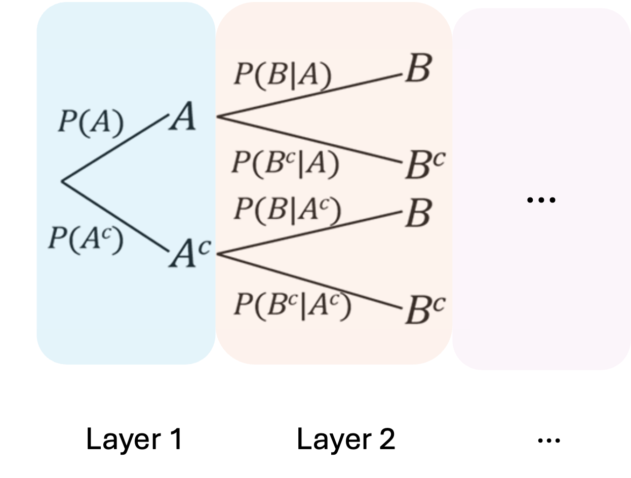
Fig. 4.14 A general tree diagram; the superscript \(^c\) is another notation for complement.

A tree diagram is constructed using the following rules:

A. Layers

The different stages are organized into vertical layers. The first vertical layer describes all events that happen during the first stage. The second layer describe all events that happen in the second stage, and the process is repeated if there are more than two stages.

B. Nodes

Each node represents an event conditional on all previous nodes. Since the first layer does not have any previous node, this is the only layer which involves unconditional events.

C. Branches

The set of branches stemming from a single node must cover all scenarios that can happen given the previous path of nodes. On each branch leading to a node, we write the conditional probability of that node given all previous nodes.

Why is a Tree Diagram Convenient?

• It provides a comprehensive picture of an experiment with many components.

• It allows us to view the general multiplication rule graphically, since the probability of a path can be computed by multiplying all the conditional probabilities along the path.

  In a two-layer tree diagram, for example, \(P(A' \cap B')\) can be computed by

  

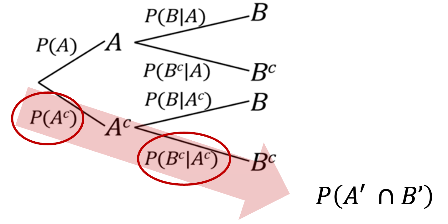
  Fig. 4.15 Computing a path probability using a tree diagram

Tree diagrams will also play a crucial role in illustrating important concepts such as the law of total probability in the following sections.

Example💡: Drawing a Tree Diagram

Glen and Jia are going to Indianapolis for one day this weekend. They are twice as likely to go on Sunday as they are on Friday, and three times as likely to go on Saturday as they are on Friday. There is a 45% chance of rain on Friday, a 25% chance of rain on Saturday, and a 30% chance of rain on Sunday.

1. Draw a complete tree diagram to represent this situation.

   Step 1: Define the notation

   • \(Fri, Sat, Sun\): events representing which day they go to Indianapolis

   • \(R\): the event that it rains during their trip

   • \(R'\): the event that it does not rain during their trip

   Step 2: Find the unknown probabilities

   Given that they are twice as likely to go on Sunday as on Friday, and three times as likely to go on Saturday as on Friday, we can write:

   \[P(Sun) = 2P(Fri) \hspace{0.2cm}\text{ and }\hspace{0.2cm} P(Sat) = 3P(Fri).\]

   Since they will go on exactly one of the three days:

   \[\begin{split}1 &= P(Fri) + P(Sat) + P(Sun) \\ &= P(Fri) + 3P(Fri) + 2P(Fri) = 6P(Fri)\\\end{split}\]

   Therefore, \(P(Fri) = 1/6\), and

   \[P(Sat) = 3P(Fri) = 1/2 \hspace{0.2cm}\text{ and }\hspace{0.2cm} P(Sun) = 2P(Fri) = 1/3.\]

   Step 3: Organize other building blocks

   We know the conditional probabilities from the weather forecasts.

   \[\begin{split}P(R|Fri) &= 0.45 \\ P(R|Sat) &= 0.25 \\ P(R|Sun) &= 0.30\end{split}\]

   Using the complement rule, we can also find:

   \[\begin{split}P(R'|Fri) = 1 - P(R|Fri)&= 0.55 \\ P(R'|Sat) = 1 - P(R|Sat)&= 0.75 \\ P(R'|Sun) = 1 - P(R|Sun)&= 0.70\end{split}\]

   Step 4: Draw the diagram

   The set of events for which we do not have any conditional probabilities should go in the first layer.

   

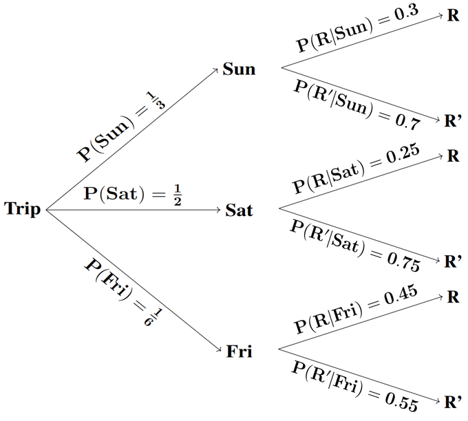
   Fig. 4.16 The tree diagram for the Indianapolis problem

2. Find the probability that they go to Indianapolis on Sunday and it does not rain.

   \[P(R' \cap Sun) = P(Sun)P(R'|Sun) = (1/3)(0.70) = 7/30.\]

4.3.4. Bringing It All Together

Key Takeaways 📝

1. Conditional probability \(P(A|B)\) represents the probability of event A occurring, given that event B occurs, and is calculated as \(P(A ∩ B)/P(B)\).

2. When we condition on an event \(B\), we effectively restrict our sample space to only the outcomes in \(B\), creating a new probability measure within this reduced space.

3. The general multiplication rule \(P(A \cap B) = P(A|B) P(B)\) allows us to find the probability of intersections using conditional probabilities.

4. Tree diagrams provide a systematic way to organize and calculate probabilities in multi-stage experiments, with the probability of each path found by multiplying conditional probabilities along branches.

5. When solving conditional probability problems, clearly define the events, identify what is known, and determine what needs to be calculated before applying the appropriate formulas.

4.3.5. Exercises

These exercises develop your skills in computing and interpreting conditional probabilities, using the general multiplication rule, and constructing tree diagrams.

Exercise 1: Conditional Probability from a Table

A semiconductor company tests chips from two production lines. The following table shows the results of testing 500 chips:

Table 4.1 Chip Quality by Production Line

	Pass	Fail	Total
Line A	180	20	200
Line B	270	30	300
Total	450	50	500

Let \(A\) = “chip is from Line A”, \(B\) = “chip is from Line B”, \(P\) = “chip passes”, and \(F\) = “chip fails.”

1. Calculate \(P(P|A)\) — the probability a chip passes given it’s from Line A.

2. Calculate \(P(P|B)\) — the probability a chip passes given it’s from Line B.

3. Calculate \(P(A|F)\) — the probability a chip is from Line A given it failed.

4. Calculate \(P(F|A)\) and verify that \(P(F|A) = 1 - P(P|A)\).

5. Are the events “Pass” and “from Line A” independent? Justify your answer.

Solution

Part (a): P(P|A)

Using the conditional probability formula:

\[P(P|A) = \frac{P(P \cap A)}{P(A)} = \frac{180/500}{200/500} = \frac{180}{200} = 0.90\]

Interpretation: 90% of chips from Line A pass inspection.

Part (b): P(P|B)

\[P(P|B) = \frac{P(P \cap B)}{P(B)} = \frac{270/500}{300/500} = \frac{270}{300} = 0.90\]

Interpretation: 90% of chips from Line B also pass inspection.

Part (c): P(A|F)

\[P(A|F) = \frac{P(A \cap F)}{P(F)} = \frac{20/500}{50/500} = \frac{20}{50} = 0.40\]

Interpretation: Given a chip failed, there’s a 40% probability it came from Line A.

Part (d): P(F|A) and Verification

\[P(F|A) = \frac{P(F \cap A)}{P(A)} = \frac{20/500}{200/500} = \frac{20}{200} = 0.10\]

Verify: \(P(F|A) = 1 - P(P|A) = 1 - 0.90 = 0.10\) ✓

This works because, given Line A, the chip either passes or fails (complement rule within the conditional space).

Part (e): Independence Check

Two events are independent if \(P(P|A) = P(P)\).

• \(P(P|A) = 0.90\)

• \(P(P) = \frac{450}{500} = 0.90\)

Since \(P(P|A) = P(P)\), yes, “Pass” and “from Line A” are independent.

Knowing a chip is from Line A doesn’t change the probability it passes. Both lines have the same 90% pass rate.

---

Exercise 2: Distinguishing Related Probabilities

A cybersecurity team analyzes network traffic. Based on historical data:

• \(P(\text{Attack}) = 0.05\) — 5% of connections are malicious attacks

• \(P(\text{Flagged}) = 0.08\) — 8% of connections trigger a security alert

• \(P(\text{Flagged} \cap \text{Attack}) = 0.04\) — 4% of connections are both attacks AND flagged

Calculate and interpret each of the following:

1. \(P(\text{Flagged} | \text{Attack})\) — Given a connection is an attack, what’s the probability it gets flagged?

2. \(P(\text{Attack} | \text{Flagged})\) — Given a connection is flagged, what’s the probability it’s actually an attack?

3. \(P(\text{Attack} | \text{Flagged}')\) — Given a connection is NOT flagged, what’s the probability it’s an attack?

4. Which probability from parts (a)-(c) represents the system’s “detection rate”? Which represents the “precision” (positive predictive value)?

Solution

Part (a): P(Flagged | Attack)

\[P(\text{Flagged} | \text{Attack}) = \frac{P(\text{Flagged} \cap \text{Attack})}{P(\text{Attack})} = \frac{0.04}{0.05} = 0.80\]

Interpretation: 80% of actual attacks are detected (flagged). This is the sensitivity or true positive rate.

Part (b): P(Attack | Flagged)

\[P(\text{Attack} | \text{Flagged}) = \frac{P(\text{Flagged} \cap \text{Attack})}{P(\text{Flagged})} = \frac{0.04}{0.08} = 0.50\]

Interpretation: When a connection is flagged, there’s only a 50% chance it’s an actual attack. The other 50% are false alarms.

Part (c): P(Attack | Flagged’)

First, find the needed probabilities:

• \(P(\text{Flagged}') = 1 - 0.08 = 0.92\)

• \(P(\text{Attack} \cap \text{Flagged}') = P(\text{Attack}) - P(\text{Attack} \cap \text{Flagged}) = 0.05 - 0.04 = 0.01\)

\[P(\text{Attack} | \text{Flagged}') = \frac{P(\text{Attack} \cap \text{Flagged}')}{P(\text{Flagged}')} = \frac{0.01}{0.92} \approx 0.0109\]

Interpretation: About 1.09% of unflagged connections are actually attacks that slipped through (missed detections).

Part (d): Classification Terminology

• Detection rate (sensitivity): \(P(\text{Flagged} | \text{Attack}) = 0.80\) from part (a)

• Precision (positive predictive value): \(P(\text{Attack} | \text{Flagged}) = 0.50\) from part (b)

Note: The detection rate and precision can be quite different! High detection doesn’t guarantee high precision if there are many false alarms.

---

Exercise 3: General Multiplication Rule

An aerospace engineer is analyzing a two-stage rocket system. Let:

• \(S_1\) = “Stage 1 succeeds”

• \(S_2\) = “Stage 2 succeeds”

Historical data shows:

• \(P(S_1) = 0.95\)

• \(P(S_2 | S_1) = 0.92\) — Stage 2 success rate given Stage 1 succeeded

• \(P(S_2 | S_1') = 0.10\) — Stage 2 success rate given Stage 1 failed

1. Calculate \(P(S_1 \cap S_2)\) — the probability both stages succeed.

2. Calculate \(P(S_1' \cap S_2)\) — the probability Stage 1 fails but Stage 2 succeeds anyway.

3. Calculate \(P(S_1' \cap S_2')\) — the probability both stages fail.

4. Verify that \(P(S_1 \cap S_2) + P(S_1 \cap S_2') + P(S_1' \cap S_2) + P(S_1' \cap S_2') = 1\).

Solution

Part (a): P(S₁ ∩ S₂)

Using the general multiplication rule:

\[P(S_1 \cap S_2) = P(S_1) \cdot P(S_2 | S_1) = 0.95 \times 0.92 = 0.874\]

Part (b): P(S₁’ ∩ S₂)

\[P(S_1' \cap S_2) = P(S_1') \cdot P(S_2 | S_1') = (1 - 0.95) \times 0.10 = 0.05 \times 0.10 = 0.005\]

Part (c): P(S₁’ ∩ S₂’)

First, find \(P(S_2' | S_1') = 1 - P(S_2 | S_1') = 1 - 0.10 = 0.90\)

\[P(S_1' \cap S_2') = P(S_1') \cdot P(S_2' | S_1') = 0.05 \times 0.90 = 0.045\]

Part (d): Verification

First, find \(P(S_1 \cap S_2')\):

\(P(S_2' | S_1) = 1 - P(S_2 | S_1) = 1 - 0.92 = 0.08\)

\(P(S_1 \cap S_2') = P(S_1) \cdot P(S_2' | S_1) = 0.95 \times 0.08 = 0.076\)

Now sum all four mutually exclusive outcomes:

\[P(S_1 \cap S_2) + P(S_1 \cap S_2') + P(S_1' \cap S_2) + P(S_1' \cap S_2')\]

\[= 0.874 + 0.076 + 0.005 + 0.045 = 1.000 \checkmark\]

These four outcomes form a partition of the sample space (every launch results in one of these four scenarios).

---

Exercise 4: Tree Diagram Construction

A tech company uses a two-stage interview process. Based on historical data:

• 60% of candidates pass the technical screening (Stage 1)

• Of those who pass the technical screening, 70% pass the behavioral interview (Stage 2)

• Of those who fail the technical screening, 20% are given a second chance and pass the behavioral interview

Let \(T\) = “passes technical screening” and \(B\) = “passes behavioral interview.”

1. Draw a complete tree diagram showing all possible paths with their probabilities.

2. Calculate the probability that a candidate passes both stages.

3. Calculate the probability that a candidate passes the behavioral interview (regardless of technical screening result).

4. Given that a candidate passed the behavioral interview, what is the probability they also passed the technical screening?

Solution

Part (a): Tree Diagram

                [Start]
               /       \
       P(T)=0.6         P(T')=0.4
           /               \
         [T]               [T']
        /   \             /    \
P(B|T)=0.7  P(B'|T)=0.3  P(B|T')=0.2  P(B'|T')=0.8
     /         \            /            \
   [B]        [B']        [B]           [B']
    |           |          |              |
 0.42        0.18       0.08           0.32

Path probabilities:

• P(T ∩ B) = 0.6 × 0.7 = 0.42

• P(T ∩ B’) = 0.6 × 0.3 = 0.18

• P(T’ ∩ B) = 0.4 × 0.2 = 0.08

• P(T’ ∩ B’) = 0.4 × 0.8 = 0.32

Part (b): P(T ∩ B)

From the tree diagram, multiplying along the top-left path:

\[P(T \cap B) = P(T) \cdot P(B|T) = 0.6 \times 0.7 = 0.42\]

Part (c): P(B)

A candidate can pass the behavioral interview through two paths:

1. Pass technical AND pass behavioral: \(P(T \cap B) = 0.42\)

2. Fail technical AND pass behavioral: \(P(T' \cap B) = 0.08\)

These paths are mutually exclusive, so:

\[P(B) = P(T \cap B) + P(T' \cap B) = 0.42 + 0.08 = 0.50\]

Part (d): P(T | B)

Using the conditional probability formula:

\[P(T|B) = \frac{P(T \cap B)}{P(B)} = \frac{0.42}{0.50} = 0.84\]

Interpretation: Given that a candidate passed the behavioral interview, there’s an 84% chance they also passed the technical screening.

---

Exercise 5: Conditional Probability with Cards

Two cards are drawn from a standard 52-card deck without replacement.

1. What is the probability that both cards are aces?

2. What is the probability that the second card is an ace, given that the first card is an ace?

3. What is the probability that exactly one of the two cards is an ace?

4. What is the probability that at least one card is an ace?

Solution

Part (a): Both Cards are Aces

Let \(A_1\) = “first card is ace” and \(A_2\) = “second card is ace”

Using the general multiplication rule:

\[P(A_1 \cap A_2) = P(A_1) \cdot P(A_2 | A_1)\]

• \(P(A_1) = \frac{4}{52}\) (4 aces out of 52 cards)

• \(P(A_2 | A_1) = \frac{3}{51}\) (after drawing one ace, 3 aces remain out of 51 cards)

\[P(A_1 \cap A_2) = \frac{4}{52} \times \frac{3}{51} = \frac{12}{2652} = \frac{1}{221} \approx 0.0045\]

Part (b): P(A₂ | A₁)

This was computed above:

\[P(A_2 | A_1) = \frac{3}{51} = \frac{1}{17} \approx 0.0588\]

Part (c): Exactly One Ace

“Exactly one” = (first is ace AND second is not) OR (first is not ace AND second is ace)

Path 1: First ace, second not ace

\[P(A_1 \cap A_2') = P(A_1) \cdot P(A_2' | A_1) = \frac{4}{52} \times \frac{48}{51} = \frac{192}{2652}\]

Path 2: First not ace, second is ace

\[P(A_1' \cap A_2) = P(A_1') \cdot P(A_2 | A_1') = \frac{48}{52} \times \frac{4}{51} = \frac{192}{2652}\]

\[P(\text{exactly one ace}) = \frac{192}{2652} + \frac{192}{2652} = \frac{384}{2652} = \frac{32}{221} \approx 0.1448\]

Part (d): At Least One Ace

Use the complement: \(P(\text{at least one}) = 1 - P(\text{no aces})\)

\[P(A_1' \cap A_2') = P(A_1') \cdot P(A_2' | A_1') = \frac{48}{52} \times \frac{47}{51} = \frac{2256}{2652}\]

\[P(\text{at least one ace}) = 1 - \frac{2256}{2652} = \frac{396}{2652} = \frac{33}{221} \approx 0.1493\]

Verification: P(exactly one) + P(both aces) should equal P(at least one):

\(\frac{32}{221} + \frac{1}{221} = \frac{33}{221}\) ✓

---

Exercise 6: Sequential Testing

A quality control process tests electronic components in sequence. Each component has a 90% probability of passing, and tests are independent.

1. If 3 components are tested, what is the probability all three pass?

2. What is the probability that the first failure occurs on the third component tested?

3. What is the probability that at least one of the three components fails?

4. A batch is accepted if at least 2 out of 3 components pass. What is the probability the batch is accepted?

Solution

Let \(P(\text{Pass}) = 0.9\) and \(P(\text{Fail}) = 0.1\) for each component.

Part (a): All Three Pass

Since tests are independent:

\[P(\text{all pass}) = 0.9 \times 0.9 \times 0.9 = 0.9^3 = 0.729\]

Part (b): First Failure on Third Component

This means: Pass, Pass, Fail

\[P(\text{PPF}) = 0.9 \times 0.9 \times 0.1 = 0.081\]

Part (c): At Least One Fails

Use complement: \(P(\text{at least one fails}) = 1 - P(\text{all pass})\)

\[P(\text{at least one fails}) = 1 - 0.729 = 0.271\]

Part (d): Batch Accepted (At Least 2 Pass)

“At least 2 pass” = (exactly 2 pass) OR (all 3 pass)

All 3 pass: \(P(\text{PPP}) = 0.729\)

Exactly 2 pass (one fails): The failure can occur in position 1, 2, or 3:

• FPP: \(0.1 \times 0.9 \times 0.9 = 0.081\)

• PFP: \(0.9 \times 0.1 \times 0.9 = 0.081\)

• PPF: \(0.9 \times 0.9 \times 0.1 = 0.081\)

\(P(\text{exactly 2 pass}) = 3 \times 0.081 = 0.243\)

\[P(\text{batch accepted}) = 0.729 + 0.243 = 0.972\]

---

4.3.6. Additional Practice Problems

True/False Questions (1 point each)

1. \(P(A|B)\) is always equal to \(P(B|A)\).

   Ⓣ or Ⓕ

2. If \(P(A|B) = P(A)\), then events A and B are independent.

   Ⓣ or Ⓕ

3. For any events A and B with \(P(B) > 0\), \(P(A|B) = \frac{P(A \cap B)}{P(B)}\).

   Ⓣ or Ⓕ

4. The general multiplication rule states \(P(A \cap B) = P(A) \cdot P(B)\).

   Ⓣ or Ⓕ

5. In a tree diagram, the probability of a complete path is found by adding the probabilities along the branches.

   Ⓣ or Ⓕ

6. \(P(A|B) + P(A'|B) = 1\).

   Ⓣ or Ⓕ

Multiple Choice Questions (2 points each)

7. If \(P(A) = 0.4\), \(P(B) = 0.5\), and \(P(A \cap B) = 0.2\), what is \(P(A|B)\)?

   Ⓐ 0.2

   Ⓑ 0.4

   Ⓒ 0.5

   Ⓓ 0.8

8. If \(P(A) = 0.3\), \(P(B|A) = 0.6\), what is \(P(A \cap B)\)?

   Ⓐ 0.18

   Ⓑ 0.30

   Ⓒ 0.50

   Ⓓ 0.90

9. A box contains 5 red and 3 blue balls. Two balls are drawn without replacement. What is the probability that the second ball is red, given that the first ball was blue?

   Ⓐ 5/8

   Ⓑ 5/7

   Ⓒ 4/7

   Ⓓ 3/8

10. If \(P(A|B) = 0.7\) and \(P(B) = 0.4\), what is \(P(A \cap B)\)?

    Ⓐ 0.175

    Ⓑ 0.28

    Ⓒ 0.40

    Ⓓ 0.70

Answers to Practice Problems

True/False Answers:

1. False — \(P(A|B)\) and \(P(B|A)\) are generally different. Example: P(Heart|Red) = 1/2, but P(Red|Heart) = 1.

2. True — This is one definition of independence. If knowing B doesn’t change the probability of A, the events are independent.

3. True — This is the definition of conditional probability.

4. False — The general multiplication rule is \(P(A \cap B) = P(A|B) \cdot P(B)\). The formula \(P(A) \cdot P(B)\) only works for independent events.

5. False — The probability of a complete path is found by multiplying (not adding) the probabilities along the branches. This is the general multiplication rule applied sequentially.

6. True — Within the conditional space of B, events A and A’ are complements. Given B occurs, either A occurs or A’ occurs (but not both).

Multiple Choice Answers:

7. Ⓑ — \(P(A|B) = \frac{P(A \cap B)}{P(B)} = \frac{0.2}{0.5} = 0.4\)

8. Ⓐ — Using the general multiplication rule: \(P(A \cap B) = P(A) \cdot P(B|A) = 0.3 \times 0.6 = 0.18\)

9. Ⓑ — After removing one blue ball, 7 balls remain (5 red, 2 blue). \(P(\text{Red}_2 | \text{Blue}_1) = \frac{5}{7}\)

10. Ⓑ — Using the general multiplication rule: \(P(A \cap B) = P(A|B) \cdot P(B) = 0.7 \times 0.4 = 0.28\)