Slides 📊
9.1. Introduction to Statistical Inference
After developing the foundational tools of probability theory, exploring random variables, and understanding sampling distributions, we have finally arrived at the core of statistical practice: statistical inference. This exciting chapter marks our transition from describing uncertainty to making decisions under uncertainty—the essence of statistics as a discipline.
Road Map 🧭
Recall the relationship between a population parameter and its estimator. Estimator yields estimates that vary from sample to sample, and their behavior is described by the sampling distribution.
Select an optimal estimator out of many candidates by evaluating their distributional properties. Know the definitions of bias and variance, and use them appropriately as selection criteria. Be able to compute bias for some simple estimators.
Know the definition of Minimum Variance Unbiased Estimator (MVUE).
9.1.1. From Population Parameters to Estimators
In statistical research, we aim to understand certain characteristics of a population that are fixed but unknown to us. These characteristics, called parameters, include:
The population mean (\(\mu\)),
The population variance (\(\sigma^2\)), and
Other quantities describing the population’s distribution.
The fundamental challenge we face is that examining every member of a population is typically impractical or impossible, even though doing so would be required to determine these characteristics with certainty. Instead, we rely on a representative sample to make inferences about the population and specify how uncertain we are about the result.
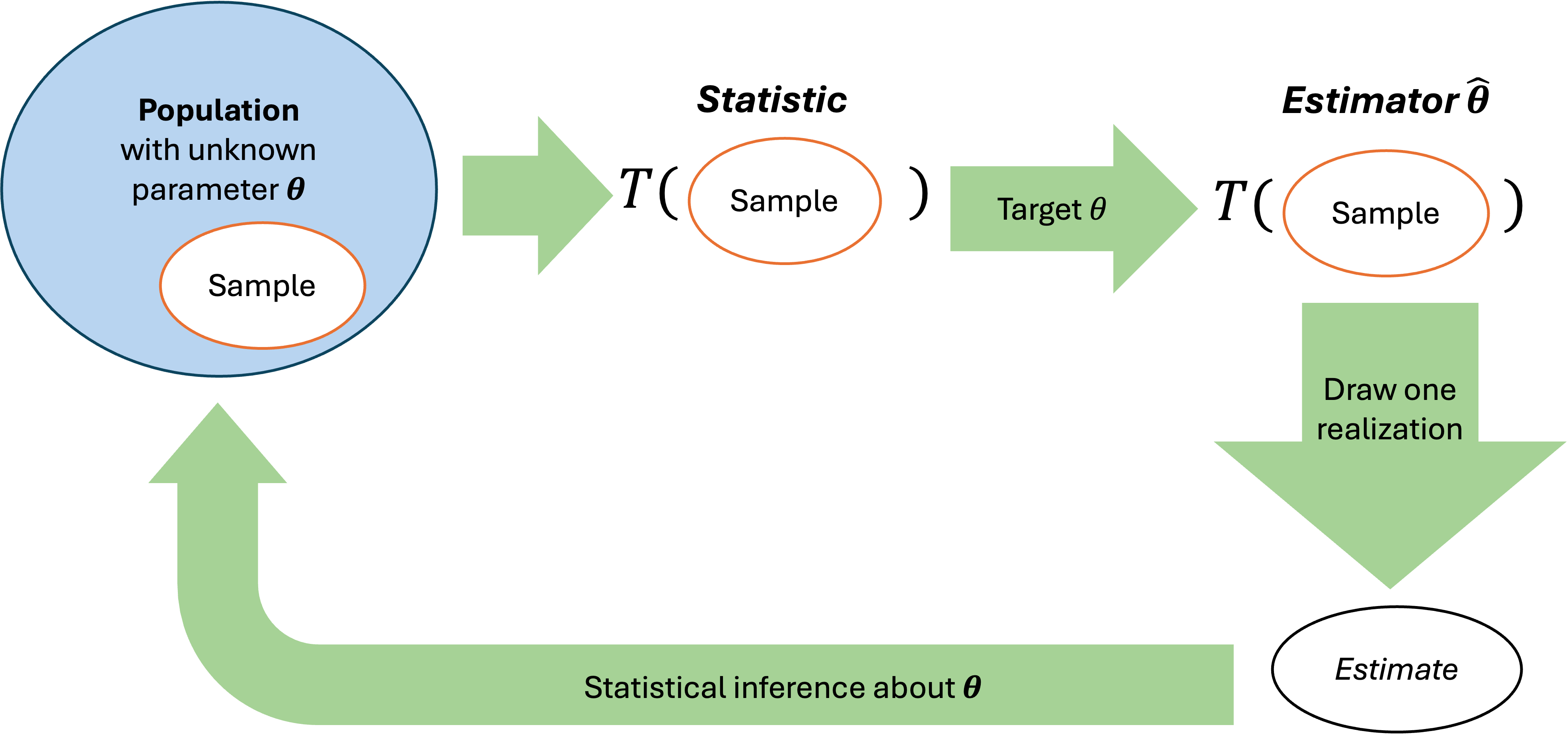
Fig. 9.1 Relationship of Parameters, estimators, and estimates
Point Estimators and Estimates
An estimator is a random variable which contains instructions on how to use sample data to calculate an estimate of a population parameter. When an estimator is designed to yield a single numerical value as an outcome, it is called a point estimator. The single-valued outcome is called a point estimate.
Example💡: \(\bar{X}\) is a Point Estimator of \(\mu\)
One possible point estimator of the population mean \(\mu\) is the sample mean \(\bar{X}\). Its definition contains instructions on the calculation procedure—adding all observed values and dividing by the sample size. A point estimate \(\bar{x}\) is obtained as a single concrete numerical value (e.g., \(\bar{x} = 42.7\)) by applying these instructions to an observed sample.
A Parameter Has Many Point Estimators
There are many different ways to guess a parameter value using data. For example, we can choose to estimate the population mean \(\mu\) with
The sample mean \(\bar{X}\) (the typical choice),
The sample median \(\tilde{X}\) (for symmetric distributions whose true mean and true median are equal, this is reasonable),
The mean of all data points except \(m\) most extreme values, etc.
It is easy to generate many reasonable candidates. The key question is, then: What objective criteria can we use to determine which estimator is better than others?
Recall from Chapter 7 that each estimator has its own distribution, called the sampling distribution. To answer the question, we focus on two key properties of the sampling distribution: bias and variance. For the remainder of this section, we use \(\theta\) (Greek letter “theta”) to denote a population parameter, and \(\hat{\theta}\) (“theta hat”) for an estimator of \(\theta\).
9.1.2. Evaluating Estimators
Bias: Does the Estimator Target the Right Value?
The bias of an estimator measures whether it systematically overestimates or underestimates the parameter of interest. It is mathematically defined as
An estimator \(\hat{\theta}\) is unbiased if \(\text{Bias}(\hat{\theta})=0\), or equivalently, if its expected value equals the parameter it aims to estimate:
Example 💡: Is the Sample Mean Unbiased?
We know that \(\mathbb{E}[\bar{X}] = \mu\). So the sample mean \(\bar{X}\) is an unbiased estimator of \(\mu\).
Variance: How Precise is the Estimator?
The variance of an estimator quantifies the spread of its sampling distribution—essentially how much the estimator fluctuates from sample to sample. Lower variance indicates greater precision and reliability.
Minimum-Variance Unbiased Estimator (MVUE)
When choosing from a set of unbiased estimators, we typically prefer the one with the smaller variance, as this reduces the expected “distance” between the estimate and the true parameter. An ideal estimator is called minimum-variance unbiased estimator (MVUE)—that is, an estimator with the smallest possible variance among all unbiased estimators for a given parameter.
Whether an estimator is MVUE depends on the population distribution, and proving this property generally requires advanced theoretical tools. Nonetheless, we will encounter several examples as we explore the properties of key estimators.
Bias-Variance Tradeoff
An unbiased estimator is not always a better choice than a biased estimator. If an estimator is slightly biased but has a significantly lower variance than its unbiased competitor, then there may be situations where the former is more practical. In fact, bias and variance often exhibit a trade-off relationship; reducing bias in an estimator may increase its variance, and vice versa. We should always take the degree of both bias and variance into consideration when choosing an estimator. See Figure Fig. 9.2 for a visual illustration:
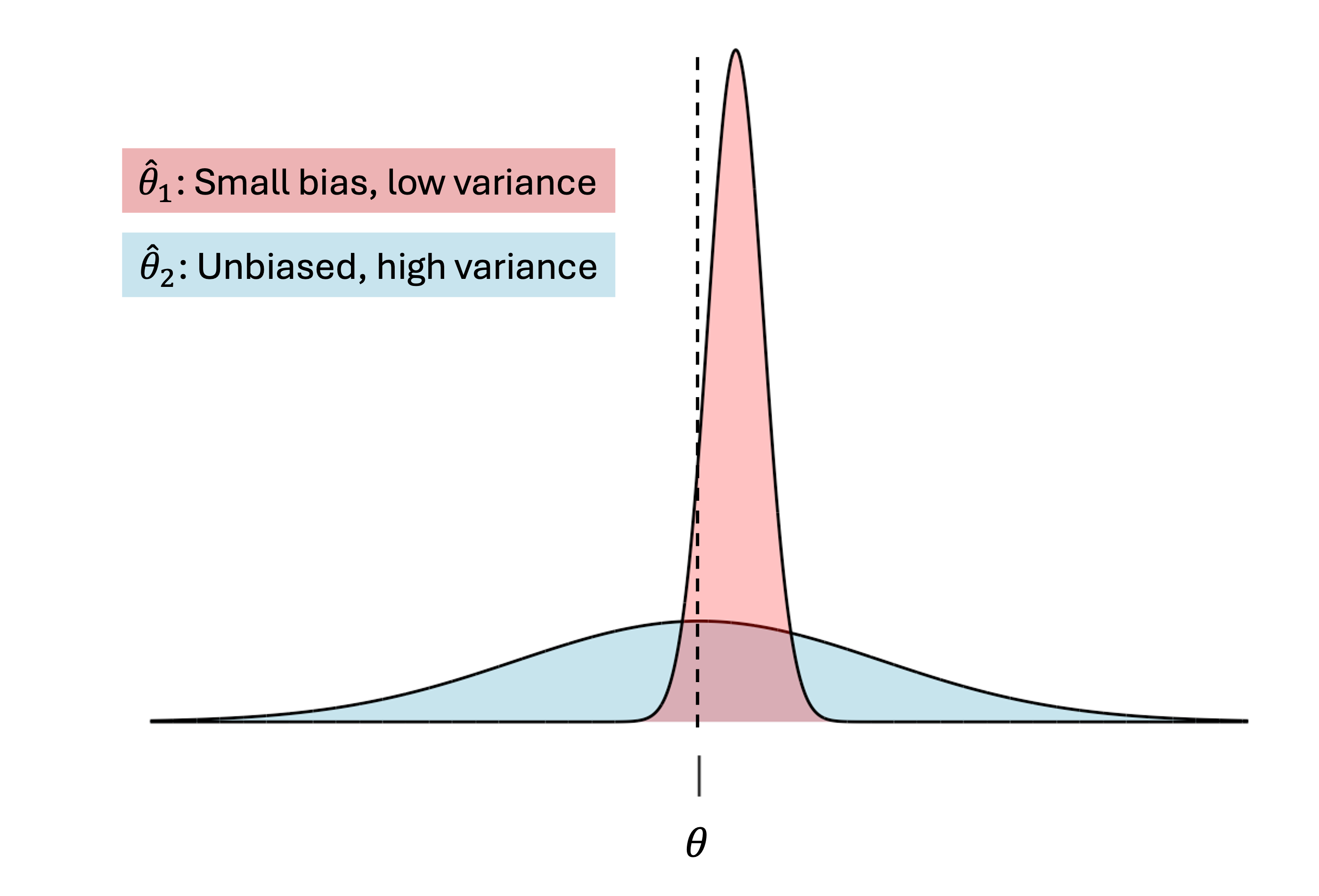
Fig. 9.2 Comparison of biased and unbiased estimators
9.1.3. Important Estimators and Their Properties
To solidify the concepts of bias and variance in estimators, let’s examine several common estimators and their properties. In all cases below, suppose \(X_1, X_2, \cdots, X_n\) form an iid sample from the same population.
A. Sample Mean for Population Mean
The sample mean \(\bar{X} = \frac{1}{n}\sum_{i=1}^{n}X_i\) serves as an estimator for the population mean \(\mu\). We know that \(\mathbb{E}[\bar{X}] = \mu\), which makes it an unbiased estimator of \(\mu\).
When sampling from a normal distribution, the sample mean is also a minimum-variance unbiased estimator (MVUE).
B. Sample Proportion for True Probability
Suppose identical trials are performed \(n\) times, and whether an event \(A\) occurs or not in each trial is recorded using Bernoulli random variables of the following form:
for \(i=1,2, \cdots, n\).
Define \(\hat{p} = \frac{1}{n}\sum_{i=1}^n I_i(A)\). Then \(\hat{p}\) is an unbiased estimator for \(P(A)\) because
This result can be used to define an unbiased estimator for an entire probability distribution.
(a) Estimating a PMF
Suppose \(X_1, X_2, \cdots, X_n\) form an iid sample of a discrete population \(X\). For each value \(x \in \text{supp}(X)\), define:
\[\hat{p}_X(x) = \frac{1}{n}\sum_{i=1}^{n}I(X_i = x),\]where \(I(X_i = x)=1\) if the \(i\)-th sample point equals \(x\), and \(0\) otherwise. Then, by the same logic as the general case, \(\hat{p}_X(x)\) is an unbiased estimator of \(p_X(x)\) for each \(x \in \text{supp}(X)\):
\[E[\hat{p}_X(x)] = p_X(x) = P(X = x).\]
(b) Estimating a CDF
For continuous random variables, we can estimate the cumulative distribution function (CDF) at any \(x \in \text{supp}(X)\) using:
\[\hat{F}_X(x) = \frac{1}{n}\sum_{i=1}^{n}I(X_i \leq x).\]\(\hat{F}_X(x)\) represents the proportion of observations less than or equal to \(x\). As another special application of the general case, this is an unbiased estimator of the true CDF \(F_X(x)\). That is,
\[E[\hat{F}_X(x)] = P(X \leq x) = F_X(x).\]
C. Sample Variance
The sample variance:
is an unbiased estimator of \(\sigma^2\). To see how, let us compute the expected value.
Add and subtract \(\mu\) inside each squared term: \((X_i - \bar{X})^2 = ((X_i - \mu) - (\bar{X} - \mu))^2\).
Using Step 1,
\[\begin{split}E[S^2]=&E\left[\frac{1}{n-1}\sum_{i=1}^n ((X_i - \mu) - (\bar{X} - \mu))^2\right]\\ =&\frac{1}{n-1}\sum_{i=1}^nE[((X_i - \mu) - (\bar{X} - \mu))^2]\\ =&\frac{1}{n-1}\sum_{i=1}^n E[(X_i - \mu)^2 -2(X_i - \mu)(\bar{X} - \mu) + (\bar{X} - \mu)^2]\\ =&\frac{1}{n-1}\sum_{i=1}^n E[(X_i - \mu)^2] -2E[(X_i - \mu)(\bar{X} - \mu)] + E[(\bar{X} - \mu)^2]\\\end{split}\]The first and third expectations are respectively the variances of \(X_i\) and \(\bar{X}\) by definition.
\[\begin{split}&E[(X_i - \mu)^2] = Var(X_i) = \sigma^2\\ &E[(\bar{X} - \mu)^2] = Var(\bar{X}) = \frac{\sigma^2}{n}\end{split}\]The expectation \(E[(X_i - \mu)(\bar{X} - \mu)]\) can be simplified to
\[\begin{split}&E[(X_i - \mu)\cdot \frac{1}{n}\sum_{j}(X_j - \mu)]= \frac{1}{n} \sum_{j=1}^n E[(X_i - \mu)(X_j - \mu)]\\ &= \frac{1}{n}E[(X_i - \mu)(X_i - \mu)] = \frac{1}{n}E[(X_i -\mu)^2] = \frac{\sigma^2}{n}\end{split}\]All terms involving indices \(j\neq i\) disappear in the final steps since \(Cov(X_i, X_j) = E[(X_i-\mu)(X_j - \mu)] =0\) due to their independence.
Substituting the results back to the final line of Step 2, we can verify that the sum simplifies to \((n-1)\sigma^2\). Therefore,
\[E[S^2] = \frac{1}{n-1} (n-1)\sigma^2 = \sigma^2.\]
This shows why we divide by \(n-1\) instead of \(n\) when computing a sample variance; this is key to making the estimator unbiased.
When sampling from normal populations, the sample variance \(S^2\) is also the MVUE for the population variance \(\sigma^2\).
Additional Exercise 💡: Sample Variance When \(\mu\) is Known
In an unrealistic situation where \(\sigma^2\) is not known but \(\mu\) is, we must incorporate the known information into our variance estimation. Show that
is an unbiased estimator of \(\sigma^2\).
The Biased Case of Sample Standard Deviation
While the sample variance \(S^2\) is an unbiased estimator of \(\sigma^2\), the sample standard deviation \(S = \sqrt{S^2}\) is a biased estimator of the population standard deviation \(\sigma\).
Its biasedness can be shown using a concept called Jensen’s inequality and the fact that the square root is a concave function. The details are beyond the scope of this course, but you are encouraged to read about the topic independently.
We still use \(S\) as our estimator for \(\sigma\) because the formula is straightforward and intuitive, while the bias is typically small, especially for larger sample sizes.
9.1.4. Bringing It All Together
In this chapter, we’ve transitioned from probability theory to statistical inference by exploring the properties of point estimators.
Key Takeaway 📝
Estimators yield estimates intended to approximate a fixed but unknown population parameter. Estimates vary from sample to sample according to their sampling distribution.
The two most important distributional characteristics of an estimator are bias and variance. Unbiased estimators target the correct parameter on average, while low-variance estimators provide more consistent results across samples.
Minimum Variance Unbiased Estimators (MVUEs) have the smallest variance among all unbiased estimators of a target parameter.
We can show that \(\bar{X}\) are \(S^2\) are unbiased estimators of their respective targets, \(\mu\) and \(\sigma^2\). When the population is normal, they are also the MVUEs.
9.2. Exercises: Introduction to Statistical Inference
Learning Objectives 🎯
These exercises will help you:
Distinguish between parameters and statistics/estimators
Understand and interpret the bias of an estimator
Understand variance and standard error as measures of estimator precision
Recognize that among unbiased estimators, lower variance is preferred
Connect sample size to the precision of the sample mean
Key Terminology
Parameter: A fixed (but often unknown) numerical value describing a population (e.g., μ, σ)
Statistic: A numerical summary computed from sample data (e.g., x̄, s)
Estimator: A statistic used to estimate a specific population parameter
Bias: \(\text{Bias}(\hat{\theta}) = E[\hat{\theta}] - \theta\); an unbiased estimator has \(E[\hat{\theta}] = \theta\)
Standard Error: The standard deviation of an estimator’s sampling distribution; for \(\bar{X}\): \(SE = \sigma/\sqrt{n}\)
9.2.1. Exercises
Exercise 1: Parameter vs Statistic Identification
For each of the following, identify whether the quantity described is a parameter (fixed, unknown population characteristic) or a statistic (calculated from sample data).
The average response time of all requests to a company’s web server over the past year.
The sample mean CPU temperature calculated from 50 randomly selected measurements during a stress test.
The proportion of all manufactured semiconductors from a production line that contain defects.
The median battery life observed in a sample of 30 laptops tested under standard conditions.
The true variance of tensile strength for all steel cables produced by a manufacturer.
The sample standard deviation of fuel efficiency measurements from 25 test vehicles.
Solution
Part (a): Parameter
This describes the average for the entire population of web server requests over the year. It is a fixed value, denoted \(\mu\).
Part (b): Statistic
This is computed from sample data (50 measurements). It will vary depending on which measurements are selected, denoted \(\bar{x}\).
Part (c): Parameter
This describes a characteristic of the entire population of semiconductors. It is a fixed proportion, denoted \(p\).
Part (d): Statistic
This is the median from a sample of 30 laptops. It is computed from sample data and would vary with different samples.
Part (e): Parameter
This is the true variance for all steel cables—the entire population. It is denoted \(\sigma^2\).
Part (f): Statistic
This is computed from a sample of 25 vehicles. It is denoted \(s\) and serves as an estimate of \(\sigma\).
Key distinction: Parameters describe populations and are typically unknown; statistics are computed from samples and serve as estimates of parameters.
Exercise 2: Understanding Estimators
A quality control engineer wants to estimate the mean diameter \(\mu\) of ball bearings produced by a manufacturing process. She considers using the following estimators based on a random sample \(X_1, X_2, \ldots, X_n\):
Estimator A: \(\hat{\mu}_A = \bar{X} = \frac{1}{n}\sum_{i=1}^{n} X_i\) (sample mean)
Estimator B: \(\hat{\mu}_B = \tilde{X}\) (sample median)
Estimator C: \(\hat{\mu}_C = \frac{X_{(1)} + X_{(n)}}{2}\) (midrange: average of min and max)
The sample mean \(\bar{X}\) is always unbiased for \(\mu\). For symmetric distributions, the median and midrange are also reasonable estimators that target the center. If multiple estimators target the same parameter, what property would you use to choose between them?
Which estimator uses all \(n\) observations in its calculation? Which uses only 2 observations?
The midrange (Estimator C) uses only the minimum and maximum values. What does this suggest about its reliability compared to the sample mean?
If you had to choose one estimator for a symmetric population, which would you choose and why?
Solution
Part (a): Choosing among estimators
When multiple estimators target the same parameter, we choose based on variance (or equivalently, standard error). Among estimators that are centered on the parameter, we prefer the one with the smallest variance because it produces estimates that are more consistently close to the true value.
Important note: \(\bar{X}\) is unbiased for \(\mu\) always. For symmetric distributions, the median and midrange are centered on the distribution’s midpoint, but finite-sample unbiasedness for \(\mu\) is not guaranteed in general.
Part (b): Observations used
Sample mean (Estimator A): Uses all \(n\) observations
Sample median (Estimator B): Uses all \(n\) observations (though only the middle values directly determine the result)
Midrange (Estimator C): Uses only 2 observations (the minimum and maximum)
Part (c): Reliability of midrange
The midrange uses only the two most extreme observations, making it:
Highly sensitive to outliers
More variable from sample to sample
Less reliable than estimators that use all the data
The sample mean “averages out” individual variations across all observations, leading to more stable (lower variance) estimates.
Part (d): Best choice
The sample mean is the best choice because:
It uses all available information (all \(n\) observations)
It is guaranteed unbiased for \(\mu\)
It has the lowest variance among common estimators for normal populations
It is not unduly influenced by any single observation (unlike the midrange)
Exercise 3: Understanding Bias
Define what it means for an estimator to be unbiased.
The sample mean \(\bar{X}\) is an unbiased estimator of the population mean \(\mu\). Explain what this means in practical terms.
Consider using the sample maximum \(X_{(n)}\) to estimate the population mean. Would this be biased or unbiased? If biased, in which direction (overestimate or underestimate)?
A researcher uses \(\frac{1}{n}\sum_{i=1}^{n}(X_i - \bar{X})^2\) instead of \(S^2 = \frac{1}{n-1}\sum_{i=1}^{n}(X_i - \bar{X})^2\) to estimate variance.
Which formula is unbiased for \(\sigma^2\)?
Does the biased formula overestimate or underestimate \(\sigma^2\) on average?
For \(n = 10\), by approximately what percentage does the biased formula underestimate \(\sigma^2\)?
Solution
Part (a): Definition of unbiased
An estimator is unbiased if its expected value equals the parameter it’s estimating:
In other words, if we could take many, many samples and compute the estimator each time, the average of all those estimates would equal the true parameter value.
Part (b): Practical meaning
Saying \(\bar{X}\) is unbiased for \(\mu\) means:
On average, the sample mean equals the population mean
There’s no systematic tendency to overestimate or underestimate
Individual samples may give \(\bar{x}\) above or below \(\mu\), but these errors balance out in the long run
\(E[\bar{X}] = \mu\) regardless of sample size
Part (c): Sample maximum as estimator
The sample maximum \(X_{(n)}\) would be a biased estimator of \(\mu\):
It would overestimate \(\mu\) on average
The maximum of a sample is typically above the center of the distribution
Only in unusual samples would the maximum be below \(\mu\)
Part (d): Variance formula comparison
(i) The formula with \(n-1\) in the denominator (\(S^2\)) is unbiased for \(\sigma^2\).
(ii) The formula with \(n\) in the denominator underestimates \(\sigma^2\) on average.
(iii) For \(n = 10\):
The biased formula gives \(\frac{n-1}{n} = \frac{9}{10} = 0.9\) of the true variance on average.
This is an underestimate of \(1 - 0.9 = 0.1 = 10\%\).
Note: This is why statistical software uses \(n-1\) by default—the correction ensures we get unbiased estimates of population variance.
Exercise 4: Why n-1 in Sample Variance?
A data scientist is analyzing algorithm runtimes and debates whether to use \(n\) or \(n-1\) in the denominator when computing sample variance.
Define both estimators:
\(\hat{\sigma}^2_{biased} = \frac{1}{n}\sum_{i=1}^{n}(X_i - \bar{X})^2\)
\(S^2 = \frac{1}{n-1}\sum_{i=1}^{n}(X_i - \bar{X})^2\)
Which one is unbiased for \(\sigma^2\)?
Express \(\hat{\sigma}^2_{biased}\) in terms of \(S^2\).
For a sample of size \(n = 5\), by what percentage does \(\hat{\sigma}^2_{biased}\) underestimate \(\sigma^2\) on average?
As \(n \to \infty\), what happens to the difference between these two estimators? Why does this make the choice less important for large samples?
Solution
Part (a): Unbiased estimator
\(S^2 = \frac{1}{n-1}\sum_{i=1}^{n}(X_i - \bar{X})^2\) is unbiased for \(\sigma^2\).
The formula with \(n\) in the denominator is biased (underestimates \(\sigma^2\)).
Part (b): Relationship
Part (c): Percentage underestimate for n = 5
The biased estimator underestimates by \(1 - 0.8 = 0.2 = 20\%\) on average.
Part (d): Large sample behavior
As \(n \to \infty\):
The two estimators become essentially identical. For \(n = 100\), the difference is only 1%. For \(n = 1000\), it’s 0.1%.
This makes the choice less important for large samples because the bias becomes negligible compared to the sampling variability.
Exercise 5: Variance of Estimators
An aerospace engineer is estimating the mean thrust \(\mu\) of a rocket engine. Two different sampling strategies yield the following estimators:
Strategy 1: Take \(n = 16\) independent measurements and compute \(\hat{\mu}_1 = \bar{X}_{16}\).
Strategy 2: Take \(n = 64\) independent measurements and compute \(\hat{\mu}_2 = \bar{X}_{64}\).
Assume the population standard deviation is \(\sigma = 200\) Newtons.
Both estimators are unbiased. Compute the variance of each estimator.
Compute the standard error (standard deviation of the sampling distribution) for each estimator.
By what factor does the standard error decrease when going from Strategy 1 to Strategy 2?
If the engineer wants to reduce the standard error by half (compared to Strategy 1), how many measurements are needed?
Solution
Part (a): Variance of each estimator
For \(\bar{X}\): \(Var(\bar{X}) = \frac{\sigma^2}{n}\)
Strategy 1 (\(n = 16\)): \(Var(\hat{\mu}_1) = \frac{200^2}{16} = \frac{40000}{16} = 2500\) N²
Strategy 2 (\(n = 64\)): \(Var(\hat{\mu}_2) = \frac{200^2}{64} = \frac{40000}{64} = 625\) N²
Part (b): Standard error
Strategy 1: \(SE_1 = \sqrt{2500} = 50\) N
Strategy 2: \(SE_2 = \sqrt{625} = 25\) N
Part (c): Factor of decrease
The standard error decreased by a factor of 2.
Note: Sample size increased by factor of 4, and \(\sqrt{4} = 2\).
Part (d): Sample size to halve SE
To halve the SE from Strategy 1 (from 50 to 25 N), we need:
This confirms Strategy 2. In general, to halve SE, quadruple the sample size.
R verification:
sigma <- 200

# Variance
sigma^2 / 16  # 2500
sigma^2 / 64  # 625

# Standard error
sigma / sqrt(16)  # 50
sigma / sqrt(64)  # 25
Exercise 6: Bias vs Variance Tradeoff (Conceptual)
Consider two estimators for a parameter \(\theta\):
Estimator A: Unbiased (hits the target on average), but high variability
Estimator B: Slightly biased (consistently a bit off), but very low variability
Draw (or describe) what the sampling distributions of these two estimators might look like relative to the true value \(\theta\).
If Estimator A gives values that range from 80 to 120 (centered at 100), and Estimator B gives values that range from 98 to 104 (centered at 102), and the true value is \(\theta = 100\), which estimator would you prefer for a single estimate? Explain.
A dartboard analogy is often used: Estimator A hits all around the bullseye (unbiased but imprecise), while Estimator B consistently hits the same spot slightly off-center (biased but precise). Which pattern would give you a better score on average?
In practice, why do statisticians often prefer unbiased estimators even when a biased estimator might occasionally be more accurate?
Solution
Part (a): Sampling distributions
Estimator A: A wide, spread-out distribution centered exactly at \(\theta = 100\). Values could be far from 100 in either direction, but they average to 100.
Estimator B: A narrow, concentrated distribution centered at 102 (slightly off from \(\theta = 100\)). Values are consistently close to 102, never exactly hitting 100.
Part (b): Preference for single estimate
Estimator A (80-120, centered at 100): Could give you anything from 80 to 120. Highly unpredictable.
Estimator B (98-104, centered at 102): Will give you something between 98 and 104. Very predictable, but always slightly high.
For a single estimate, Estimator B might be preferred because:
The worst case (104) is closer to 100 than Estimator A’s worst cases (80 or 120)
Even though it’s biased, the estimates are all “in the ballpark”
Estimator A has a wide range where individual estimates could be quite wrong
Part (c): Dartboard analogy
Estimator A (all around bullseye): Some darts hit close to center, but many are far away
Estimator B (consistent off-center): All darts land in a tight cluster, just not at the center
For overall accuracy, Estimator B would typically score better because the consistent small miss beats the highly variable hits and misses of Estimator A.
Part (d): Why prefer unbiased estimators
Systematic errors compound: In repeated use or when combining estimates, bias doesn’t cancel out, but random errors do
Interpretability: Unbiased estimates are easier to explain and trust
Unknown bias: We often don’t know the size of the bias, so we can’t correct for it
Statistical theory: Many confidence interval and hypothesis testing procedures assume unbiased estimators
Scientific standards: Many fields require unbiased methods for credibility
Exercise 7: Standard Error of the Sample Mean
A software company tests \(n = 100\) randomly selected user sessions to estimate the mean session duration. Based on historical data, the population standard deviation is known to be \(\sigma = 8\) minutes.
What is the standard error of the sample mean?
If the company increases the sample size to \(n = 400\), what is the new standard error?
By what factor did the standard error decrease when \(n\) increased from 100 to 400?
How large should \(n\) be to achieve a standard error of at most 0.5 minutes?
A colleague suggests that doubling the sample size will halve the standard error. Is this correct? Explain.
Solution
Given: \(\sigma = 8\) minutes
Part (a): SE with n = 100
Part (b): SE with n = 400
Part (c): Factor of decrease
The SE decreased by a factor of 2. Note: \(n\) increased by a factor of 4, and \(\sqrt{4} = 2\).
Part (d): Required n for SE ≤ 0.5
Need at least n = 256 sessions.
Part (e): Doubling sample size
Incorrect. Doubling the sample size reduces the standard error by a factor of \(\sqrt{2} \approx 1.41\), not by half.
To halve the standard error, you must quadruple the sample size because:
If you want \(SE_{new} = \frac{1}{2} SE_{old}\), then \(\sqrt{n_{new}} = 2\sqrt{n_{old}}\), so \(n_{new} = 4n_{old}\).
R verification:
sigma <- 8

# SE for different n
sigma / sqrt(100)   # 0.8
sigma / sqrt(400)   # 0.4

# Required n for SE = 0.5
(sigma / 0.5)^2     # 256
Exercise 8: True/False Conceptual Questions
Determine whether each statement is True or False. Provide a brief justification.
An unbiased estimator will always give the exact value of the parameter.
The sample mean \(\bar{X}\) is an unbiased estimator of the population mean \(\mu\) for any sample size.
If two estimators are both unbiased, the one with smaller variance is generally preferred.
The sample variance \(S^2 = \frac{1}{n-1}\sum(X_i - \bar{X})^2\) is an unbiased estimator of \(\sigma^2\).
Increasing sample size reduces the variance of the sample mean.
A biased estimator is always worse than an unbiased estimator.
Solution
Part (a): False
Being unbiased means the estimator is correct on average across many samples. Any single sample’s estimate may be above or below the true parameter. Unbiased ≠ perfect.
Part (b): True
\(E[\bar{X}] = \mu\) regardless of the population distribution or sample size. This is a fundamental property of the sample mean.
Part (c): True
Among unbiased estimators, lower variance means estimates are more consistently close to the true parameter value. We want precision along with accuracy.
Part (d): True
The formula \(S^2 = \frac{1}{n-1}\sum(X_i - \bar{X})^2\) is unbiased for \(\sigma^2\) regardless of the underlying distribution, as long as the observations are independent with the same variance.
Part (e): True
\(Var(\bar{X}) = \frac{\sigma^2}{n}\), which decreases as \(n\) increases. Larger samples give more precise estimates.
Part (f): False
A biased estimator with very low variance might actually give estimates that are, on average, closer to the true value than an unbiased estimator with high variance. The “best” estimator depends on the context and what properties matter most.
Exercise 9: Application - Sensor Calibration
A biomedical engineer is calibrating a blood pressure sensor. She tests the sensor against a known reference standard with true value \(\mu = 120\) mmHg. After \(n = 20\) independent measurements, she records the following data:
118.2, 121.5, 119.8, 122.1, 117.9, 120.4, 123.2, 118.6, 121.0, 119.5,
120.8, 117.5, 122.8, 119.2, 121.7, 118.9, 120.1, 122.4, 119.6, 120.5
Compute the sample mean \(\bar{x}\) and sample standard deviation \(s\).
The observed “bias” in this sample is \(\bar{x} - \mu\). Calculate this value. Does the sensor appear to overestimate or underestimate?
If the engineer wanted to correct for this observed bias, how might she adjust future readings?
Can we conclude from this single sample that the estimator \(\bar{X}\) is biased? Explain why or why not.
Solution
Part (a): Summary statistics
measurements <- c(118.2, 121.5, 119.8, 122.1, 117.9, 120.4, 123.2, 118.6,
                  121.0, 119.5, 120.8, 117.5, 122.8, 119.2, 121.7, 118.9,
                  120.1, 122.4, 119.6, 120.5)

mean(measurements)  # 120.285
sd(measurements)    # 1.657
Sample mean: \(\bar{x} = 120.285\) mmHg
Sample standard deviation: \(s = 1.657\) mmHg
Part (b): Observed bias
The sensor appears to be slightly overestimating the true pressure in this specific sample.
Part (c): Calibration correction
If the engineer assumes this observed difference of 0.285 mmHg is a consistent hardware bias, she could apply a simple offset correction to future readings:
Suggestion: Applying this correction now is a statistical trap. Because this is based on a single small sample, we do not know if 0.285 mmHg is the true underlying bias or just random sampling noise. A proper engineering approach requires two steps:
Conduct a much larger study at this 120 mmHg baseline just to detect if the bias statistically exists (distinguishing a true signal from random noise).
If it does exist, conduct several follow-up studies across many conditions (e.g., varying true pressures, temperatures, and humidity) to determine if the bias is a flat offset, a proportional percentage error, or an environmental artifact, before permanently adjusting the sensor.
Part (d): Can we conclude bias?
No, we absolutely cannot conclude the estimator is biased based on this one test.
Bias is a property of the sampling distribution, not a single sample.
The standard error of our estimate is \(SE = s/\sqrt{n} = 1.657/\sqrt{20} \approx 0.37\) mmHg.
The observed deviation (0.285) is less than 1 Standard Error away from the true mean. It is entirely consistent with ordinary random sampling variability.
To assess true hardware bias, the engineer would need the larger sample size described in (c) to shrink the SE, or repeated independent calibration tests to see if the average of many \(\bar{x}\) values systematically misses \(\mu\).
9.2.2. Additional Practice Problems
True/False Questions (1 point each)
The population mean \(\mu\) is a random variable.
Ⓣ or Ⓕ
Different samples from the same population will yield different values of \(\bar{x}\).
Ⓣ or Ⓕ
An estimator with zero bias will always produce estimates equal to the true parameter.
Ⓣ or Ⓕ
The standard error of \(\bar{X}\) depends on the sample size.
Ⓣ or Ⓕ
Among unbiased estimators, we prefer the one with the smallest variance.
Ⓣ or Ⓕ
Quadrupling the sample size will halve the standard error.
Ⓣ or Ⓕ
Multiple Choice Questions (2 points each)
Which of the following is a parameter?
Ⓐ The average height of 50 randomly selected students
Ⓑ The standard deviation of test scores for all students in a school
Ⓒ The sample proportion of defective items in a shipment
Ⓓ The median income from a survey of 1,000 households
The sample variance formula uses \(n-1\) instead of \(n\) in the denominator because:
Ⓐ It makes calculations easier
Ⓑ It produces an unbiased estimator of \(\sigma^2\)
Ⓒ It produces larger variance estimates
Ⓓ It is required for the normal distribution
If \(\sigma = 20\) and \(n = 100\), the standard error of \(\bar{X}\) is:
Ⓐ 20
Ⓑ 2
Ⓒ 0.2
Ⓓ 200
To reduce the standard error by a factor of 3, the sample size must be increased by a factor of:
Ⓐ 3
Ⓑ 6
Ⓒ 9
Ⓓ \(\sqrt{3}\)
Which quantity describes the precision of an estimator?
Ⓐ Bias
Ⓑ Variance
Ⓒ Expected value
Ⓓ Sample size
An unbiased estimator with variance 100 vs. a biased estimator (bias = 2) with variance 25. Which has smaller expected squared error from the true parameter?
Ⓐ The unbiased estimator (expected squared error = 100)
Ⓑ The biased estimator (expected squared error = 29)
Ⓒ They are equal
Ⓓ Cannot be determined
Answers to Practice Problems
True/False Answers:
False — \(\mu\) is a fixed (though unknown) population constant, not a random variable.
True — Due to sampling variability, different samples produce different sample means.
False — Zero bias means correct on average over many samples, not correct every time.
True — \(SE = \sigma/\sqrt{n}\), which depends on \(n\).
True — Lower variance means more precision (estimates cluster more tightly around the parameter).
True — \(SE \propto 1/\sqrt{n}\), so if \(n\) increases by 4, SE decreases by \(\sqrt{4} = 2\).
Multiple Choice Answers:
Ⓑ — “All students in a school” indicates this is a population characteristic, making it a parameter.
Ⓑ — The \(n-1\) correction (Bessel’s correction) makes \(S^2\) unbiased for \(\sigma^2\).
Ⓑ — \(SE = \sigma/\sqrt{n} = 20/\sqrt{100} = 20/10 = 2\).
Ⓒ — To reduce SE by factor of 3, need \(\sqrt{n_{new}/n_{old}} = 3\), so \(n_{new}/n_{old} = 9\).
Ⓑ — Variance measures how spread out the estimates are around their expected value (precision).
Ⓑ — Expected squared error = Variance + Bias². Unbiased: 100 + 0 = 100. Biased: 25 + 4 = 29. The biased estimator has smaller expected squared error.