Final Exam — Spring 2026: Worked Solutions

Exam Information

Course: STAT 350 — Introduction to Statistics

Semester: Spring 2026

Total Points: 150 + 15 (Extra Credit) = 165

Time Allowed: 120 minutes

Coverage: Cumulative (Chapters 1–13); primary emphasis on Chapters 12–13, with Chapters 1–7 weighted more heavily than Chapters 8–11 among the earlier material

Problem	Total Possible	Topic
Problem 1 (True/False, 2 pts each)	20	Linear Transformations, Independence, Poisson, Uniform, PDF Interpretation, ANOVA Methods, F-test, Regression Units, CI Duality, Normality Assumption
Problem 2 (Multiple Choice, 3 pts each)	18	Venn Diagrams, Exponential Memoryless, Conditional Normal, Bonferroni, ANOVA Assumptions, Scatter Plots/Correlation
Problem 3	24	Piecewise PDF/CDF, Variance of Transformation
Problem 4	26	Total Probability, Bayes’ Rule, Binomial Distribution
Problem 5	40	One-Way ANOVA, Tukey HSD
Problem 6	37	Simple Linear Regression, LINE Assumptions, Prediction, Confidence Interval
Total	150 (+ 15 Extra Credit)

Exam PDF

Solution Key PDF

—

Problem 1 — True/False (20 points, 2 pts each)

Question 1.1 (2 pts)

A sensor records temperatures in Celsius. A data analyst converts every observation to Fahrenheit using \(F = 1.8C + 32\).

The sample standard deviation of the Fahrenheit data is exactly 1.8 times the sample standard deviation of the Celsius data.

Solution

Answer: TRUE

For a linear transformation \(Y = aX + b\), the standard deviation transforms as \(s_Y = |a|\,s_X\). Here \(a = 1.8\) and \(b = 32\), so \(s_F = 1.8\,s_C\). The additive constant does not affect spread.

Question 1.2 (2 pts)

A mechanical engineer classifies each manufactured part as exactly one of three grades: \(A\) (premium), \(B\) (standard), or \(C\) (substandard). The historical probability for the classification to each grade are \(P(A) = 0.3\), \(P(B) = 0.6\), and \(P(C) = 0.1\).

Events \(A\) and \(C\) are dependent.

Solution

Answer: TRUE

Since each part receives exactly one grade, \(A\) and \(C\) are mutually exclusive: \(P(A \cap C) = 0\). For independence we would need \(P(A \cap C) = P(A)\,P(C) = 0.3 \times 0.1 = 0.03 \neq 0\). Because the product rule fails, \(A\) and \(C\) are dependent.

Question 1.3 (2 pts)

During an NFL season, a sports analytics team tracks all reported injuries sustained by a single team per game quarter, including those not immediately apparent to viewers such as minor strains and aggravations recorded on the official injury report. It has been historically observed that the team averages approximately 1.4 reported injuries per quarter across all games. However, detailed records reveal that injury rates in the 4th quarter are consistently higher than in the 1st quarter, as cumulative fatigue increases injury risk throughout a game.

A single \(\text{Poisson}(\lambda = 1.4)\) model applied uniformly across all four quarters would violate an assumption of the Poisson process.

Solution

Answer: TRUE

A Poisson process requires a constant rate \(\lambda\) over the interval of interest. If the injury rate is higher in the 4th quarter than in the 1st quarter, the rate is not constant across quarters. Applying a single \(\lambda = 1.4\) uniformly ignores this non-constant rate and violates the homogeneity assumption.

Question 1.4 (2 pts)

Two CNC machines produce bolts whose diameters (in mm) follow continuous uniform distributions. Machine A produces bolts with diameters following \(\text{Uniform}(9.5, 10.5)\) and Machine B produces bolts with diameters following \(\text{Uniform}(9.8, 10.8)\).

The probability that Machine A produces a bolt with a diameter between 9.8 and 10.0 is the same as the probability that Machine B does.

Solution

Answer: TRUE

For a \(\text{Uniform}(a, b)\) distribution, \(P(c < X < d) = (d - c)/(b - a)\) when \([c, d] \subseteq [a, b]\).

\[P(9.8 < X_A < 10.0) = \frac{10.0 - 9.8}{10.5 - 9.5} = \frac{0.2}{1.0} = 0.2\]

\[P(9.8 < X_B < 10.0) = \frac{10.0 - 9.8}{10.8 - 9.8} = \frac{0.2}{1.0} = 0.2\]

Both probabilities equal 0.2.

Question 1.5 (2 pts)

A quality engineer models the lifespan of a sensor component using a continuous distribution. She computes \(f_X(500) = 0.003\), where \(f_X\) is the PDF of the lifespan in hours.

Therefore the engineer is certain that a lifespan of 500 hours is very rare.

Solution

Answer: FALSE

The value \(f_X(500) = 0.003\) is a probability density, not a probability. For a continuous random variable, \(P(X = 500) = 0\) regardless of the PDF value. Density values can exceed 1 or be very small without directly indicating how “rare” a specific value is. Only the area under the PDF (an integral) gives a probability.

Question 1.6 (2 pts)

A one-way ANOVA with 5 groups produces a significant \(F\)-test.

If the researcher wants to compare all 10 possible pairs of means, Dunnett’s method is more appropriate than Tukey’s method.

Solution

Answer: FALSE

Dunnett’s method is designed for comparing each treatment group to a single control group, not for all pairwise comparisons. With 5 groups and \(\binom{5}{2} = 10\) pairwise comparisons, Tukey’s HSD is the appropriate method. Dunnett’s would only cover \(k - 1 = 4\) comparisons (each treatment vs. the control).

Question 1.7 (2 pts)

In a one-way ANOVA, if the between-group variability is large relative to the within-group variability,

then the \(F\)-test statistic will tend to be large, giving more evidence against the null hypothesis that all population means are equal.

Solution

Answer: TRUE

The ANOVA \(F\)-statistic is \(F = \text{MSA}/\text{MSE}\), where MSA captures between-group variability and MSE captures within-group variability. When between-group variability is large relative to within-group variability, \(F\) is large, pushing the \(p\)-value toward zero and providing stronger evidence against \(H_0\).

Question 1.8 (2 pts)

A biostatistician plans to fit a simple linear regression line to predict male adults’ height using their femur bone length. Both variables are measured in inches in the original data. Before fitting a regression line, the unit has changed to millimeters for universal applications in medical fields.

The \(p\)-value of a regression slope remains constant even after the unit change.

Solution

Answer: TRUE

Both \(X\) (femur length) and \(Y\) (height) are converted by the same factor: \(1\;\text{inch} = 25.4\;\text{mm}\). The slope transforms as:

\[b_{1,\text{mm}} = \frac{\Delta Y_{\text{mm}}}{\Delta X_{\text{mm}}} = \frac{25.4\,\Delta Y_{\text{in}}}{25.4\,\Delta X_{\text{in}}} = b_{1,\text{in}}\]

Since the slope estimate is unchanged, its standard error, \(t\)-statistic, and \(p\)-value are all unchanged.

Question 1.9 (2 pts)

Suppose that \((-3, 4)\) is a 95% confidence interval for \(\beta_0\) in a simple linear regression. For some constant \(c\), we perform hypothesis testing \(H_a\colon \beta_0 \neq c\) at \(\alpha = 0.05\).

We reject the null hypothesis if \(c\) is within the confidence interval.

Solution

Answer: FALSE

The CI–test duality says: at the same confidence level and significance level, we fail to reject \(H_0\colon \beta_0 = c\) when \(c\) falls inside the confidence interval. We reject \(H_0\) when \(c\) falls outside the interval. The statement reverses the direction.

Question 1.10 (2 pts)

A materials engineer fits a simple linear regression to predict tensile strength (\(Y\)) from carbon content (\(X\)) in steel alloys. Before checking residuals, the engineer examines the distribution of \(Y\) values alone and finds them to be strongly right-skewed.

The normality assumption of the simple linear regression model is violated.

Solution

Answer: FALSE

The normality assumption in simple linear regression applies to the error terms (equivalently, the residuals), not to the marginal distribution of \(Y\). Even if \(Y\) is right-skewed marginally, the conditional distribution \(Y \mid X = x\) (and therefore the errors) can still be normal. The skewness in \(Y\) may simply reflect the distribution of \(X\) values. Normality must be assessed from a residual plot or normal Q–Q plot of residuals, not from the marginal distribution of \(Y\).

—

Problem 2 — Multiple Choice (18 points, 3 pts each)

Question 2.1 (3 pts)

A software quality team reviews 200 applications for two categories of defects before deployment. Let \(M = \{\text{has memory leak issues}\}\) and \(B = \{\text{has performance bottleneck issues}\}\).

The Venn diagram shows the number of applications in each region.

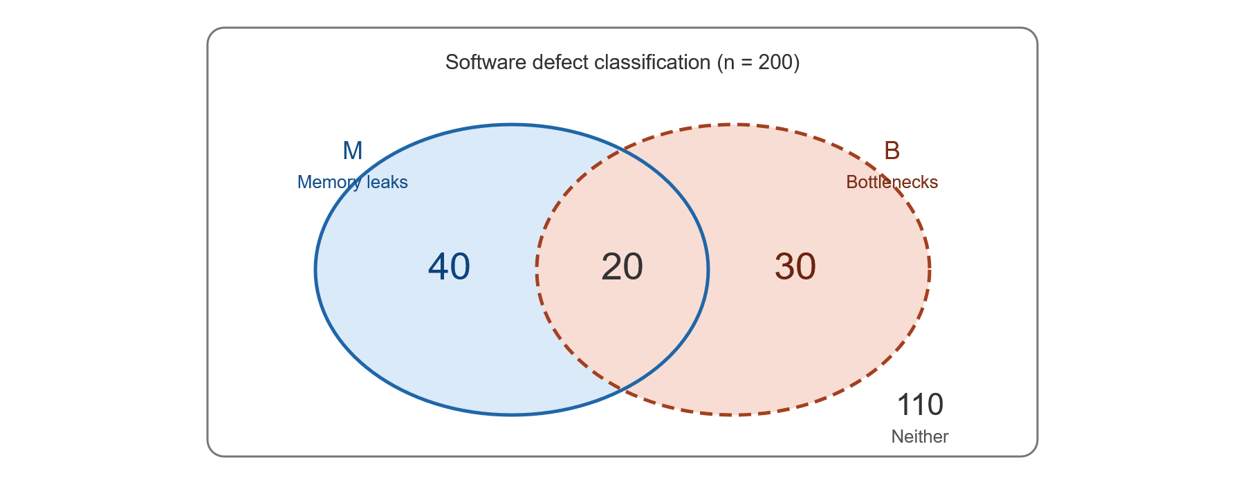
Which of the following counts is computed correctly? (\(|\cdot|\) denotes size of set)

• 1. \(|M' \cap B'| = 110\)

• 2. \(|M' \cap B| = 180\)

• 3. \(|M \cap B'| = 30\)

• 4. \(|M \cup B'| = 150\)

Solution

Answer: (A)

From the Venn diagram: \(|M| = 40 + 20 = 60\), \(|B| = 20 + 30 = 50\), \(|M \cap B| = 20\), neither \(= 110\).

• (A) \(|M' \cap B'|\) = applications with neither defect \(= 110\). CORRECT.

• (B) \(|M' \cap B|\) = applications with bottleneck only \(= 30 \neq 180\).

• (C) \(|M \cap B'|\) = applications with memory leak only \(= 40 \neq 30\).

• (D) \(|M \cup B'| = |M| + |B'| - |M \cap B'| = 60 + 150 - 40 = 170 \neq 150\).

Question 2.2 (3 pts)

A semiconductor fabrication line experiences random equipment faults. The time (in hours) between faults follows an Exponential distribution with rate \(\lambda = 0.5\) per hour. The line has been running fault-free for at least 6 hours.

What is the probability it continues to run fault-free for at least two more hours?

• 1. 0.0183

• 2. 0.0498

• 3. 0.1353

• 4. 0.3679

• 5. 0.6321

Solution

Answer: (D)

By the memoryless property of the Exponential distribution:

\[P(T > 8 \mid T > 6) = P(T > 2) = e^{-0.5 \times 2} = e^{-1} \approx 0.3679\]

pexp(2, rate = 0.5, lower.tail = FALSE)
# [1] 0.3679

Question 2.3 (3 pts)

The response time (in milliseconds) of a web application follows a Normal distribution with \(\mu = 250\) and \(\sigma = 20\). A request is classified as “slow” if it takes more than 230 ms.

Given that a request is slow, what is the probability it takes more than 280 ms? Fractions are shown for readability. In R, these would be written using the / operator.

• 1. pnorm(280, mean = 250, sd = 20, lower.tail = FALSE)

• 2. pnorm(280, mean = 250, sd = 20, lower.tail = FALSE) / pnorm(230, mean = 250, sd = 20, lower.tail = TRUE)

• 3. (pnorm(280, mean = 250, sd = 20, lower.tail = TRUE) - pnorm(230, mean = 250, sd = 20, lower.tail = TRUE)) / pnorm(230, mean = 250, sd = 20, lower.tail = FALSE)

• 4. pnorm(280, mean = 250, sd = 20, lower.tail = FALSE) / pnorm(230, mean = 250, sd = 20, lower.tail = FALSE)

Solution

Answer: (D)

We need \(P(X > 280 \mid X > 230)\). By the definition of conditional probability:

\[P(X > 280 \mid X > 230) = \frac{P(X > 280 \cap X > 230)}{P(X > 230)} = \frac{P(X > 280)}{P(X > 230)}\]

since \(\{X > 280\} \subseteq \{X > 230\}\). In R:

pnorm(280, 250, 20, lower.tail = FALSE) / pnorm(230, 250, 20, lower.tail = FALSE)
# [1] 0.07941

Question 2.4 (3 pts)

A one-way ANOVA with 4 groups is significant, and the researcher wants to compare all possible pairs of means using Bonferroni. What is the Bonferroni-adjusted significance level for each comparison if the family-wise error rate is set to 0.05?

• 1. 0.0500

• 2. 0.0250

• 3. 0.0125

• 4. 0.0083

• 5. 0.0050

Solution

Answer: (D)

With \(k = 4\) groups, the number of pairwise comparisons is \(C = \binom{4}{2} = 6\). The Bonferroni-adjusted significance level is:

\[\alpha_{\text{adj}} = \frac{\alpha}{C} = \frac{0.05}{6} \approx 0.0083\]

Question 2.5 (3 pts)

Which of the following is not required for a traditional one-way ANOVA?

• 1. Independent random samples from each population

• 2. Equal population variances across groups

• 3. Each of the \(k\) populations is normally distributed, or sample means are approximately normally distributed

• 4. Equal sample sizes in all groups

Solution

Answer: (D)

The three assumptions for one-way ANOVA are: (1) independence — samples are independent random samples from their respective populations; (2) normality — each population is normally distributed, or sample sizes are large enough for the CLT to apply; and (3) equal variances (homoscedasticity) — the population variances are equal across all groups. Equal sample sizes are not required, although balanced designs are preferred for robustness and power.

Question 2.6 (3 pts)

A dataset consists of one response variable and four explanatory variables (Variables 1–4). For each explanatory variable, a scatter plot is drawn against the response variable. Select the two explanatory variables whose sample correlation coefficient \(r\) with the response variable is closest to zero.

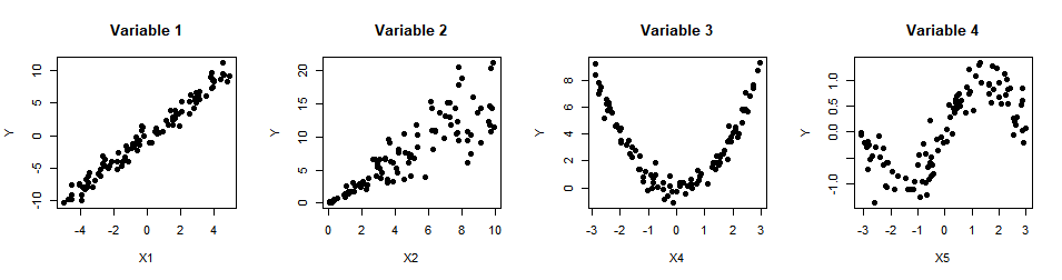
• 1. Variables 1 & 2

• 2. Variables 2 & 3

• 3. Variables 2 & 4

• 4. Variables 3 & 4

• 5. None — all four variables have strong sample correlations with the response variable.

Solution

Answer: (D)

The sample correlation coefficient \(r\) measures the strength and direction of a linear relationship:

• Variable 1: Strong positive linear trend → \(|r|\) is high.

• Variable 2: Strong positive linear trend with moderate spread → \(|r|\) is high.

• Variable 3: U-shaped (quadratic) pattern — a strong nonlinear relationship, but virtually no linear trend → \(|r| \approx 0\).

• Variable 4: Scattered cloud with no clear pattern → \(|r| \approx 0\).

Variables 3 and 4 have sample correlations closest to zero.

—

Problem 3 Setup

A utility company, Earl Energy, is known for long customer service wait times. Let \(X\) denote the waiting time (in hours) until a customer is connected to the next available representative. The probability density function (pdf) and cumulative distribution function (cdf) of \(X\) are given below.

\[\begin{split}f_X(x) = \begin{cases} 0, & x < 0 \\[4pt] \dfrac{1}{2}\,x^2\,e^{-x}, & x \geq 0 \end{cases}\end{split}\]

\[\begin{split}F_X(x) = \begin{cases} 0, & x < 0 \\[4pt] 1 - \dfrac{1}{2}\,e^{-x}\,(x^2 + 2x + 2), & x \geq 0 \end{cases}\end{split}\]

Problem 3 — Piecewise PDF/CDF (24 points)

Question 3a (10 pts)

What is the probability that a customer waits for more than 30 minutes?

Solution

30 minutes = 0.5 hours. We need \(P(X > 0.5) = 1 - F_X(0.5)\):

\[P\!\left(X > \tfrac{1}{2}\right) = 1 - F_X\!\left(\tfrac{1}{2}\right) = 1 - \left[1 - \tfrac{1}{2}\,e^{-1/2}\left(\left(\tfrac{1}{2}\right)^2 + 2\!\cdot\!\tfrac{1}{2} + 2\right)\right]\]

\[= \tfrac{1}{2}\,e^{-1/2}\left(\tfrac{1}{4} + 1 + 2\right) = \tfrac{1}{2}\,e^{-1/2} \cdot \tfrac{13}{4} = e^{-1/2} \cdot \tfrac{13}{8} \approx \boxed{0.9856}\]

1 - (1 - 0.5 * exp(-0.5) * (0.5^2 + 2*0.5 + 2))
# [1] 0.9856

Question 3b (14 pts)

Find the variance of a rate \(\dfrac{1}{X}\) given that \(E\!\left[\dfrac{1}{X}\right] = 0.5\).

Solution

Using \(\text{Var}(1/X) = E[1/X^2] - \left(E[1/X]\right)^2\):

\[E\!\left[\frac{1}{X^2}\right] = \int_0^{\infty} \frac{1}{x^2} \cdot \frac{1}{2}\,x^2\,e^{-x}\,dx = \frac{1}{2}\int_0^{\infty} e^{-x}\,dx = \frac{1}{2}\]

Therefore:

\[\text{Var}\!\left(\frac{1}{X}\right) = E\!\left[\frac{1}{X^2}\right] - \left(E\!\left[\frac{1}{X}\right]\right)^2 = \frac{1}{2} - \left(\frac{1}{2}\right)^2 = \frac{1}{2} - \frac{1}{4} = \boxed{\frac{1}{4} = 0.25}\]

—

Problem 4 Setup

A software team uses Claude Code to assist with code commits. Each commit is independently classified as either routine or novel. A routine commit is routed to Configuration A, and a novel commit is routed to Configuration B. Each commit independently has a 20% probability of being novel (Configuration B) and an 80% probability of being routine (Configuration A).

During a particular week, the team makes 25 commits. Each commit is automatically and independently tested for bugs. The probability that a Configuration A commit contains a bug is 0.05, and the probability that a Configuration B commit contains a bug is 0.30.

Problem 4 — Total Probability, Bayes’ Rule, Binomial (26 points)

Question 4a (10 pts)

A single commit is selected at random from the week’s 25 commits. What is the probability that it contains a bug?

Solution

By the Law of Total Probability:

\[P(\text{Bug}) = P(\text{Bug} \mid A)\,P(A) + P(\text{Bug} \mid B)\,P(B)\]

\[= 0.05 \times 0.8 + 0.30 \times 0.2 = 0.04 + 0.06 = \boxed{0.1}\]

Question 4b (10 pts)

A single commit from the week is found to contain a bug. What is the probability it was handled by Configuration B?

Solution

By Bayes’ Rule:

\[P(B \mid \text{Bug}) = \frac{P(\text{Bug} \mid B)\,P(B)}{P(\text{Bug})} = \frac{0.30 \times 0.2}{0.1} = \frac{0.06}{0.1} = \boxed{0.6}\]

Question 4c (6 pts)

Find the expected number and standard deviation of bugs found in Configuration B during the week.

Solution

Let \(X_B\) denote the number of bugs found in Configuration B during the week. Each of the 25 commits independently has probability \(P(\text{Bug} \cap B) = P(\text{Bug} \mid B)\,P(B) = 0.30 \times 0.20 = 0.06\) of being a Configuration B bug. Therefore:

\[X_B \sim \text{Binomial}(n = 25,\; p = 0.06)\]

\[E[X_B] = np = 25 \times 0.06 = \boxed{1.5}\]

\[\text{Var}(X_B) = np(1-p) = 25 \times 0.06 \times 0.94 = 1.41\]

\[\text{SD}(X_B) = \sqrt{1.41} \approx \boxed{1.1874}\]

—

Problem 5 Setup

An agronomist wants to compare the average plant height increase (in cm) produced by four fertilizers. A random sample of plants was assigned to each fertilizer treatment. The summary information is given below.

Group	\(n_i\)	\(\bar{x}_i\)	\(s_i\)
Fertilizer 1	10	17.80	2.05
Fertilizer 2	10	20.70	2.31
Fertilizer 3	10	19.25	2.18
Fertilizer 4	10	24.00	2.42

Problem 5 — One-Way ANOVA, Tukey HSD (40 points)

Question 5a (2 pts)

Using the summary statistics, assess whether the equal variance (homogeneity of variance) assumption appears reasonable. Show your work and state your conclusion clearly. For the rest of the problem, assume all other ANOVA assumptions are satisfied.

Solution

Check the ratio of largest to smallest sample standard deviations:

\[\frac{s_{\max}}{s_{\min}} = \frac{2.42}{2.05} \approx 1.1805 < 2\]

By the rule of thumb, the equal variance assumption is reasonable.

Question 5b (14 pts)

Complete the ANOVA table below. The Factor Sum of Squares is 211.2687, the Error Sum of Squares is 181.3266, and the \(p\)-value is \(3.351353 \times 10^{-6}\).

Solution

With \(k = 4\) groups and \(N = 40\) total observations:

\[\bar{\bar{x}} = \frac{10(17.80) + 10(20.70) + 10(19.25) + 10(24.00)}{40} = \frac{817.5}{40} = 20.4375\]

Degrees of freedom:

• Factor: \(k - 1 = 3\)

• Error: \(N - k = 36\)

• Total: \(N - 1 = 39\)

Mean Squares:

\[\text{MSA} = \frac{\text{SSA}}{k-1} = \frac{211.2687}{3} = 70.4229\]

\[\text{MSE} = \frac{\text{SSE}}{N-k} = \frac{181.3266}{36} = 5.0369\]

F-statistic:

\[F = \frac{\text{MSA}}{\text{MSE}} = \frac{70.4229}{5.0369} = 13.9815\]

Table 28 ANOVA Table

Source	df	Sum of Squares	Mean Square	\(F\)	\(\Pr(>F)\)
Factor	3	211.2687	70.4229	13.9815	\(3.35 \times 10^{-6}\)
Error	36	181.3266	5.0369
Total	39	392.5953

Question 5c (4 pts)

Provide the first two steps of the four-step one-way ANOVA hypothesis testing procedure.

Solution

Step 1 — Identify and describe the parameter(s):

Let \(\mu_1, \mu_2, \mu_3, \mu_4\) denote the true mean height increase in cm treated with Fertilizers 1, 2, 3, and 4, respectively.

Step 2 — Define the hypotheses:

\[H_0\colon \mu_1 = \mu_2 = \mu_3 = \mu_4\]

\[H_a\colon \text{At least one mean is different}\]

Question 5d (3 pts)

Which of the following R code statements returns the correct \(p\)-value?

• 1. pf(F_ts/2, df1=4, df2 = 36, lower.tail = FALSE)

• 2. pf(F_ts, df1=3, df2 = 36, lower.tail = FALSE)

• 3. pf(F_ts, df1=4, df2 = 37, lower.tail = TRUE)

• 4. pf(F_ts, df1=3, df2 = 36, lower.tail = TRUE)

• 5. 2*pf(F_ts, df1=4, df2 = 40, lower.tail = FALSE)

Solution

Answer: (B)

The ANOVA \(F\)-test is always upper-tailed. The \(p\)-value is \(P(F > F_{\text{TS}})\) with numerator df \(= k - 1 = 3\) and denominator df \(= N - k = 36\):

pf(F_ts, df1 = 3, df2 = 36, lower.tail = FALSE)
# [1] 3.351353e-06

Question 5e (8 pts)

The calculated \(p\)-value is \(3.35 \times 10^{-6}\). At a significance level of \(\alpha = 0.05\), state your formal decision and conclusion in the context of the problem.

Solution

Since the \(p\)-value \(= 3.35 \times 10^{-6} < 0.05 = \alpha\), we have evidence to reject \(H_0\).

The data does give strong support (\(p\)-value \(= 3.35 \times 10^{-6}\)) to the claim that at least one of the fertilizers produces a true mean height increase (in centimeters) that differs from at least one other.

Question 5f (4 pts)

Based on your conclusion in part (e), is it appropriate to proceed to pairwise comparisons such as Tukey’s HSD? Briefly explain.

Solution

Yes. Since we rejected the null hypothesis, we have evidence that at least one pair of means differs. To determine which means are different, a post-hoc analysis such as Tukey’s HSD should be conducted.

Question 5g (5 pts)

The following Tukey HSD results were obtained. Construct a graphical display based on these results, and briefly state which fertilizer appears to have the largest population mean plant height increase and provide justification.

Comparison	diff	lwr	upr	p adj
Fertilizer 2 − Fertilizer 1	2.9000	0.1969	5.6031	0.0306
Fertilizer 3 − Fertilizer 1	1.4500	−1.2531	4.1531	0.4807
Fertilizer 4 − Fertilizer 1	6.2000	3.4969	8.9031	0.0000
Fertilizer 3 − Fertilizer 2	−1.4500	−4.1531	1.2531	0.4807
Fertilizer 4 − Fertilizer 2	3.3000	0.5969	6.0031	0.0118
Fertilizer 4 − Fertilizer 3	4.7500	2.0469	7.4531	0.0002

Solution

Significant pairs (p adj < 0.05): (2−1), (4−1), (4−2), (4−3).

Non-significant pairs (p adj ≥ 0.05): (3−1) with p = 0.4807, and (3−2) with p = 0.4807.

Underline display (groups ordered by sample mean; groups connected by the same underline are not significantly different):

Two overlapping underlines: one connecting Fertilizer 1–Fertilizer 3, and a second connecting Fertilizer 3–Fertilizer 2. Fertilizer 4 stands alone — significantly different from all others.

Fertilizer 4 appears to have the largest population mean height increase (\(\bar{x}_4 = 24.00\)), and it is significantly higher than every other fertilizer at the 5% family-wise level.

—

Problem 6 Setup

A driving school wants to estimate the monthly car insurance premium for teenage drivers who are at least 16 but under 20 years old (all with minimum-coverage policies). They randomly selected 100 teen drivers and recorded each driver’s monthly premium (in dollars) and age (in years) at enrollment. Preliminary analysis indicates a linear relationship between monthly premium (\(y\)) and age (\(x\)). The school plans to fit a simple linear regression model to provide statistical estimates of monthly premiums based on age.

\(S_{xx} = 63.797\)	\(S_{xy} = -538.3375\)	\(S_{yy} = 24069\)
\(\bar{x} = 17.5535\)	\(\bar{y} = 204.2009\)	\(n = 100\)

Problem 6 — Simple Linear Regression (37 points)

Question 6a (10 pts)

The simple linear regression model requires four assumptions. Not all assumptions are needed at every stage of the analysis pipeline.

1. State the four assumptions.

2. For each assumption, identify the stage at which it is first required: model fitting/estimation, statistical inference, or prediction intervals.

3. Explain why prediction intervals are not robust to the violation of the assumption identified in ii.

Solution

i. The four assumptions (LINE):

• Linearity: The true relationship between \(x\) and \(y\) is linear, meaning \(E[Y \mid x] = \beta_0 + \beta_1 x\). Part of model fitting/estimation.

• Independence: The error terms \(\varepsilon_1, \varepsilon_2, \ldots, \varepsilon_n\) are independent of one another. Needed for proper statistical inference and prediction intervals.

• Normality: The error terms \(\varepsilon_1, \varepsilon_2, \ldots, \varepsilon_n\) are normally distributed with zero mean. Needed for prediction intervals, though standard statistical inference (CIs and tests for \(\beta_0, \beta_1\)) can rely on the CLT.

• Equal Variance (Homoscedasticity): The variance of the errors is constant across all values of \(x\). Needed for statistical inference and prediction intervals.

ii. Stage identification:

Normality is the assumption whose violation most directly impacts prediction intervals while being somewhat robust at the inference stage (via the CLT).

iii. Why prediction intervals are not robust to normality violations:

A confidence interval for the mean response (\(E[Y \mid x_0]\)) benefits from the CLT: since the estimates of the slope and intercept are averages (weighted) of many observations, their sampling distributions become approximately normal even when the errors are not, provided \(n\) is reasonably large.

A prediction interval, however, must account for the variability of a single future observation \(Y_0 = \beta_0 + \beta_1 x_0 + \varepsilon_0\) as well as that of the estimate of the mean response. The interval’s coverage depends directly on the distribution of that individual error term \(\varepsilon_0\) — there is no averaging and no CLT to rescue us. If the errors are skewed or heavy-tailed, the interval endpoints (constructed assuming normality) will be in the wrong places, and the stated coverage probability (e.g., 95%) will be incorrect.

Question 6b (8 pts)

Assuming all assumptions are met, compute the slope \(b_1\) and the intercept \(b_0\). Write the fitted regression line \(\hat{y}\).

Solution

\[b_1 = \frac{S_{xy}}{S_{xx}} = \frac{-538.3375}{63.797} = -8.4383\]

\[b_0 = \bar{y} - b_1\,\bar{x} = 204.2009 - (-8.4383)(17.5535) = 352.3226\]

Regression line:

\[\hat{y} = 352.3226 - 8.4383\,x\]

Question 6c (8 pts)

Predict the monthly premium for a 17-year-old teen and a 13-year-old teen, respectively. Discuss the statistical validity of these predictions.

Solution

Plug in \(x = 17\) and \(x = 13\) to the regression line:

\[\hat{y}_{17} = 352.3226 - 8.4383 \times 17 = 352.3226 - 143.4511 = 208.8715\]

\[\hat{y}_{13} = 352.3226 - 8.4383 \times 13 = 352.3226 - 109.6979 = 242.6247\]

The prediction for a 17-year-old is statistically valid, because 17 falls within the range of observed ages (16 to under 20). This is an interpolation.

The prediction for a 13-year-old is not statistically valid, because 13 falls outside the observed age range. This is an extrapolation, and the linear model may not accurately reflect premiums for ages not represented in the data.

Question 6d (8 pts)

Construct a 95% confidence interval for the mean monthly premium of all 17-year-old drivers. Use the R output below, along with the summary statistics from the problem introduction and your fitted regression model.

Residual standard error: 14.12 on 98 degrees of freedom
Multiple R-squared: 0.1887, Adjusted R-squared: 0.1804
F-statistic: 22.8 on 1 and 98 DF, p-value: 6.296e-06

qt(0.025, 98, lower.tail=FALSE) [1] 1.984467	qf(0.025, 1, 98, lower.tail=FALSE) [1] 5.181823
qt(0.05, 98, lower.tail=FALSE) [1] 1.660551	qf(0.05, 1, 98, lower.tail=FALSE) [1] 3.938111

Solution

Compute the standard error of the mean prediction at \(x^* = 17\):

\[SE(\hat{y}_{17}) = s\,\sqrt{\frac{1}{n} + \frac{(x^* - \bar{x})^2}{S_{xx}}} = 14.12\,\sqrt{\frac{1}{100} + \frac{(17 - 17.5535)^2}{63.797}}\]

\[= 14.12\,\sqrt{0.01 + 0.004802} = 14.12 \times 0.12167 \approx 1.7179\]

The 95% CI is \(\hat{y}_{17} \pm t_{0.025,\,df=98} \times SE(\hat{y}_{17})\):

\[208.8715 \pm 1.984467 \times 1.7179 = 208.8715 \pm 3.4093\]

\[\approx \boxed{(205.46,\; 212.28)}\]

Question 6e (3 pts)

Which of the following statements is reasonable regarding an interval estimate for a new response \(x^*\)?

• 1. The confidence interval for \(y^*\) becomes wider if \(x^*\) moves farther away from the sample mean \(\bar{x}\).

• 2. The confidence interval for \(y^*\) becomes narrower if \(x^*\) moves farther away from the sample mean \(\bar{x}\).

• 3. The prediction interval for \(y^*\) becomes wider if \(x^*\) moves farther away from the sample mean \(\bar{x}\).

• 4. The prediction interval for \(y^*\) becomes narrower if \(x^*\) moves farther away from the sample mean \(\bar{x}\).

Solution

Answer: (C)

Both confidence intervals (for the mean response) and prediction intervals (for a new observation) contain the term \((x^* - \bar{x})^2 / S_{xx}\) inside the square root of their standard error formulas. As \(x^*\) moves farther from \(\bar{x}\), this term increases, making the interval wider. The question asks about a new response, which uses a prediction interval. Option (C) correctly describes this behavior.