Exam 1 — Spring 2025: Fully Worked Solutions

• Exam PDF

• Solution PDF

The questions below reproduce the Spring 2025 Exam 1 in full accessible text. Each problem is followed by a complete worked solution. Point values reflect the actual exam.

Table 4 Point Summary

Section	Format	Points
Problem 1 — True/False	6 questions × 2 pts	12
Problem 2 — Multiple Choice	5 questions × 3 pts	15
Problem 3 — Free Response	4 parts	26
Problem 4 — Free Response	5 parts	26
Problem 5 — Free Response	2 parts	26
Total		105

---

Problem 1: True/False (12 points, 2 points each)

Indicate the correct answer by completely filling in the appropriate circle. If you indicate your answer by any other way, you may be marked incorrect.

Question 1.1 (2 pts)

The boxplot below visually displays the summary information for a dataset.

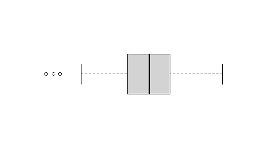
T or F: According to the boxplot above, a lower inner fence must be located between the lower whisker and the largest outlier.

Solution

Answer: TRUE

Recall how the modified boxplot is constructed:

• The lower inner fence is defined as \(Q_1 - 1.5 \times IQR\).

• The lower whisker extends left from \(Q_1\) to the smallest observed value that is still at or above the lower inner fence.

• Any data point below the lower inner fence is plotted as an explicit point (outlier).

The left-to-right arrangement is therefore:

\[\underbrace{\text{most extreme outlier}}_{\text{farthest left}} \;\cdots\; \underbrace{\text{largest outlier}}_{\text{closest to fence}} \;<\; \underbrace{\text{lower inner fence}}_{} \;\leq\; \underbrace{\text{lower whisker endpoint}}_{} \;\leq\; Q_1.\]

The lower inner fence lies between the largest outlier (to its left) and the lower whisker endpoint (to its right). The statement is TRUE.

---

Question 1.2 (2 pts)

The Binomial distribution is symmetric when

T or F: the probability of success \(p\) is close to 0 or 1.

Solution

Answer: FALSE

A \(\text{Binomial}(n, p)\) distribution is symmetric when \(p = 0.5\). When \(p = 0.5\), every outcome \(x\) and its mirror \(n - x\) are equally probable, making the PMF perfectly symmetric about \(n/2\).

When \(p\) is close to 0, the distribution is strongly right-skewed. When \(p\) is close to 1, the distribution is strongly left-skewed. The statement is FALSE.

---

Question 1.3 (2 pts)

Suppose \(Y\) is the outcome of a single roll of a 6-sided die with an unknown probability mass function having nonzero variance. The outcome for a random variable \(X\) is obtained by throwing this die once then multiplying the resulting number by 3, i.e., \(X = 3Y\). The outcome for another random variable \(Z\) is obtained by throwing the same die three times, then adding the results together, i.e., \(Z = Y_1 + Y_2 + Y_3\) where \(Y_1, Y_2, Y_3\) are independent copies of \(Y\). Then,

T or F: it follows that \(\text{Var}(X) = \text{Var}(Z)\).

Solution

Answer: FALSE

Variance of X:

\[\text{Var}(X) = \text{Var}(3Y) = 3^2\,\text{Var}(Y) = 9\,\text{Var}(Y).\]

Variance of Z:

Since \(Y_1, Y_2, Y_3\) are independent:

\[\text{Var}(Z) = \text{Var}(Y_1) + \text{Var}(Y_2) + \text{Var}(Y_3) = 3\,\text{Var}(Y).\]

Since \(\text{Var}(Y) > 0\):

\[\text{Var}(X) = 9\,\text{Var}(Y) \neq 3\,\text{Var}(Y) = \text{Var}(Z).\]

The statement is FALSE.

Intuition

Multiplying a single roll by 3 amplifies spread by \(3^2 = 9\). Adding three independent rolls grows variance only linearly (factor of 3). Despite having the same expected value, \(X\) is much more variable than \(Z\).

---

Question 1.4 (2 pts)

Let \(X\) denote a normal random variable, then regardless of the value of \(E[X]\) and \(\text{Var}(X)\),

T or F: \(P\!\left(E[X] - 2\sqrt{\text{Var}(X)} < X < E[X] + 2\sqrt{\text{Var}(X)}\right) \approx 0.95\) is always true.

Solution

Answer: TRUE

Let \(\mu = E[X]\) and \(\sigma = \sqrt{\text{Var}(X)}\). Standardize:

\[P(\mu - 2\sigma < X < \mu + 2\sigma) = P\!\left(-2 < \frac{X - \mu}{\sigma} < 2\right) = P(-2 < Z < 2),\]

where \(Z \sim N(0,1)\). From the standard normal table:

\[P(-2 < Z < 2) = \Phi(2) - \Phi(-2) = 0.9772 - 0.0228 = 0.9544 \approx 0.95.\]

This holds for any normal random variable regardless of \(\mu\) or \(\sigma\). The statement is TRUE.

---

Question 1.5 (2 pts)

Let \(X\) be an exponential random variable. Then,

T or F: the distribution of \(X\) models the probability associated with the total number of events occurring during a fixed interval of time.

Solution

Answer: FALSE

The Exponential distribution models the waiting time between successive events in a Poisson process — it is continuous, taking values in \([0, \infty)\).

The distribution that models the number of events in a fixed time interval is the Poisson distribution, which is discrete.

Table 5 Poisson vs. Exponential

Feature	Poisson(\(\lambda\))	Exponential(\(\lambda\))
Models	Number of events in fixed time	Waiting time until next event
Type	Discrete	Continuous
Mean	\(\lambda\)	\(1/\lambda\)

The statement is FALSE.

---

Question 1.6 (2 pts)

Let \(X\) be a continuous random variable with finite expected value \(\mu\) and variance \(\sigma^2\). Define a new random variable \(Y = aX + b\) where \(a, b\) are real numbers with \(a \neq 0\).

T or F: It follows that \(E[Y^2] = a^2(\sigma^2 + \mu^2) + 2ab\mu + b^2\) always holds, regardless of the distribution of \(X\).

Solution

Answer: TRUE

Expand \(Y^2 = (aX+b)^2 = a^2X^2 + 2abX + b^2\) and apply linearity of expectation:

\[E[Y^2] = a^2\,E[X^2] + 2ab\,E[X] + b^2.\]

Substitute \(E[X] = \mu\) and \(E[X^2] = \text{Var}(X) + (E[X])^2 = \sigma^2 + \mu^2\):

\[E[Y^2] = a^2(\sigma^2 + \mu^2) + 2ab\mu + b^2.\]

This follows from the definitions of expectation and variance alone — no assumptions about the distribution of \(X\) are required. The statement is TRUE.

---

Problem 2: Multiple Choice (15 points, 3 points each)

Indicate the correct answer by completely filling in the appropriate circle. If you indicate your answer by any other way, you may be marked incorrect. For each question, there is only one correct option letter choice.

Question 2.1 (3 pts)

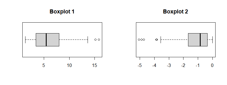
Which of the following provides the best measures of center and spread respectively, based on the boxplots below?

• (A) Boxplot 1: sample mean, interquartile range (IQR)

• (B) Boxplot 1: sample median, range

• (C) Boxplot 1: sample mean, sample standard deviation

• (D) Boxplot 2: sample median, interquartile range (IQR)

• (E) Boxplot 2: sample median, range

• (F) Boxplot 2: sample mean, sample standard deviation

Solution

Answer: (D)

Both distributions are skewed and contain outliers. The sample mean and standard deviation are non-resistant and are pulled toward extreme values. The median and IQR are resistant summaries better suited to skewed or outlier-prone data.

Only (D) correctly pairs a resistant measure of center (median) with a resistant measure of spread (IQR) for a distribution that is skewed and contains outliers.

Why the Boxplot 1 options fail:

• (A) uses the sample mean on Boxplot 1, which is pulled upward by the two upper outliers. The median would be the appropriate measure of center here.

• (B) pairs the sample median (good choice) with the range (poor choice). The range is entirely determined by the two most extreme values and is the least resistant measure of spread possible.

• (C) uses both the sample mean and standard deviation, both of which are non-resistant to the upper outliers in Boxplot 1.

Why the remaining Boxplot 2 options fail:

• (E) correctly identifies the sample median as the measure of center, but pairs it with the range, which is dominated by the four lower outliers in Boxplot 2.

• (F) uses the sample mean and standard deviation, both of which are heavily distorted by the four lower outliers visible in Boxplot 2.

---

Question 2.2 (3 pts)

Assume \(X \sim N(\mu, \sigma)\), \(Y \sim \text{Exp}(\lambda)\), and \(Z \sim \text{Bin}(n, p)\). Which of the following statements is TRUE?

• (A) For the parameters of \(X\) the ratio \(\mu/\sigma\) must be greater than 1.

• (B) For any \(y\) in the support of \(Y\) there exists an \(x\) in the support of \(X\) such that \(x = y\).

• (C) The variance of \(Y\) is the same as the mean of \(Y\).

• (D) If \(p < 0.5\), then \(Z\) can never take any values greater than \(n/2\). In other words, \(Z\) is supported only on integers strictly less than \(n/2\).

• (E) The parameter \(\lambda\) must be a positive integer.

Solution

Answer: (B)

(A) FALSE. The only constraint on normal parameters is \(\sigma > 0\). The mean \(\mu\) may be any real number, including negative values. For example, \(X \sim N(\mu = -5,\; \sigma = 10)\) is perfectly valid, giving \(\mu/\sigma = -0.5\), which is not greater than 1.

(B) TRUE. The support of \(Y \sim \text{Exp}(\lambda)\) is \([0, \infty)\). The support of \(X \sim N(\mu, \sigma)\) is all of \((-\infty, \infty)\). Since \((-\infty, \infty) \supset [0, \infty)\), every non-negative value in the support of \(Y\) is also in the support of \(X\). The statement is TRUE.

(C) FALSE. For \(Y \sim \text{Exp}(\lambda)\):

\[E[Y] = \frac{1}{\lambda}, \qquad \text{Var}(Y) = \frac{1}{\lambda^2}.\]

The claim is that \(\text{Var}(Y) = E[Y]\), i.e., \(1/\lambda^2 = 1/\lambda\). This holds only when \(\lambda = 1\). For any other value of \(\lambda\), \(\text{Var}(Y) \neq E[Y]\).

(D) FALSE. The support of \(Z \sim \text{Bin}(n,p)\) is \(\{0, 1, \ldots, n\}\) for any \(p \in (0,1)\), regardless of whether \(p < 0.5\). When \(p < 0.5\) the distribution is right-skewed, but values near \(n\) still have positive probability — for example, \(P(Z = n) = p^n > 0\).

(E) FALSE. The Exponential rate parameter \(\lambda\) must only be positive (\(\lambda > 0\)); it need not be an integer. For example, \(\lambda = 0.3\) or \(\lambda = 2.7\) are both valid.

---

Question 2.3 (3 pts)

Harry works at Hogwarts mail center. The number of owls that he receives in an hour at the center (\(X\)) follows Poisson distribution with an average hourly rate of 1. In other words, \(X \sim \text{Poisson}(\lambda = 1)\). Which of the following is not true?

• (A) The probability that Harry receives \(x\) owls in an hour is \(\dfrac{1^x e^{-1}}{x!}\).

• (B) The probability that Harry receives 1 owl in an hour is approximately 0.3679.

• (C) The probability that Harry receives 2 owls in an hour is approximately 0.1839.

• (D) The probability that Harry receives more than 2 owls in an hour is approximately 0.2642.

• (E) The probability that Harry receives 1 owl in the first hour of his shift then zero in the second hour is approximately 0.1353.

Solution

Answer: (D)

With \(\lambda = 1\), the PMF is \(P(X = x) = e^{-1}/x!\).

(A) TRUE. Substituting \(\lambda = 1\) into the Poisson PMF formula \(P(X=x) = e^{-\lambda}\lambda^x / x!\) gives \(P(X=x) = e^{-1} \cdot 1^x / x! = 1^x e^{-1} / x!\). ✓

(B) TRUE. \(P(X=1) = e^{-1}/1! = e^{-1} \approx 0.3679\).

(C) TRUE. \(P(X=2) = e^{-1}/2! = e^{-1}/2 \approx 0.1839\).

(D) NOT TRUE. Compute \(P(X > 2) = 1 - P(X \leq 2)\):

\[P(X \leq 2) = e^{-1}\!\left(1 + 1 + \tfrac{1}{2}\right) = 2.5\,e^{-1} \approx 0.9197.\]

\[P(X > 2) = 1 - 0.9197 = 0.0803 \neq 0.2642.\]

(E) TRUE. By independence of the two hours: \(P(X_1=1)\cdot P(X_2=0) = e^{-1} \cdot e^{-1} = e^{-2} \approx 0.1353\).

---

Question 2.4 (3 pts)

If \(X\) is a Poisson random variable that satisfies \(P(X=5) = P(X=7)\), then \(P(X=0) = {?}\)

• (A) \(P(X=0) = e^{0}\)

• (B) \(P(X=0) = e^{-5}\)

• (C) \(P(X=0) = e^{-7}\)

• (D) \(P(X=0) = e^{-\sqrt{35}}\)

• (E) \(P(X=0) = e^{-\sqrt{42}}\)

Solution

Answer: (E)

Set the two Poisson probabilities equal and solve for \(\lambda\):

\[\frac{e^{-\lambda}\lambda^5}{5!} = \frac{e^{-\lambda}\lambda^7}{7!}.\]

Cancel \(e^{-\lambda}\) and \(\lambda^5\) (both positive):

\[\frac{1}{5!} = \frac{\lambda^2}{7!} \implies \lambda^2 = \frac{7!}{5!} = 7 \times 6 = 42 \implies \lambda = \sqrt{42}.\]

Therefore \(P(X=0) = e^{-\lambda} = e^{-\sqrt{42}}\). The answer is (E).

---

Question 2.5 (3 pts)

In the standard Normal distribution, for any \(z > 0\), how does the probability compare between the two regions \(-z < Z < 0\) and \(0 < Z < z\)? Determine the correct symbol connecting the two probability statements below (fill in the blank).

\[P(-z < Z < 0) \quad \underline{\hspace{1cm}} \quad P(0 < Z < z)\]

• (A) \(<\)

• (B) \(>\)

• (C) \(=\)

• (D) \(\neq\)

• (E) \(\subset\)

Solution

Answer: (C)

The standard normal PDF is symmetric about zero: \(f(-t) = f(t)\) for all \(t\). Therefore:

\[P(-z < Z < 0) = \Phi(0) - \Phi(-z) = 0.5 - (1 - \Phi(z)) = \Phi(z) - 0.5,\]

\[P(0 < Z < z) = \Phi(z) - \Phi(0) = \Phi(z) - 0.5.\]

Both expressions equal \(\Phi(z) - 0.5\), so the correct symbol is \(=\).

---

Free Response Questions 3–5

Show all work, clearly label your answers, and use four decimal places.

Problem 3 (26 points)

Problem 3 Setup

In an alternative timeline where Lafayette evolved into a structured statistical metropolis, two competing academic institutions, STAT High School (STAT HS) and STAT Middle School (STAT MS), compete for control of a shared soccer field used for team practices and school games.

The field is reserved on a monthly basis, with STAT High School holding the reservation 74% of the time, independent of other months. Whenever STAT High School does not secure the reservation, it is automatically assigned to STAT Middle School.

The number of games played each month follows the distribution depicted by the probability mass functions in the figure below.

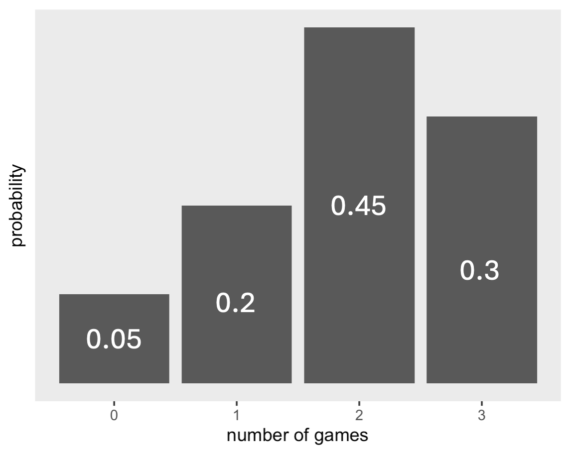
Fig. 1 STAT HS

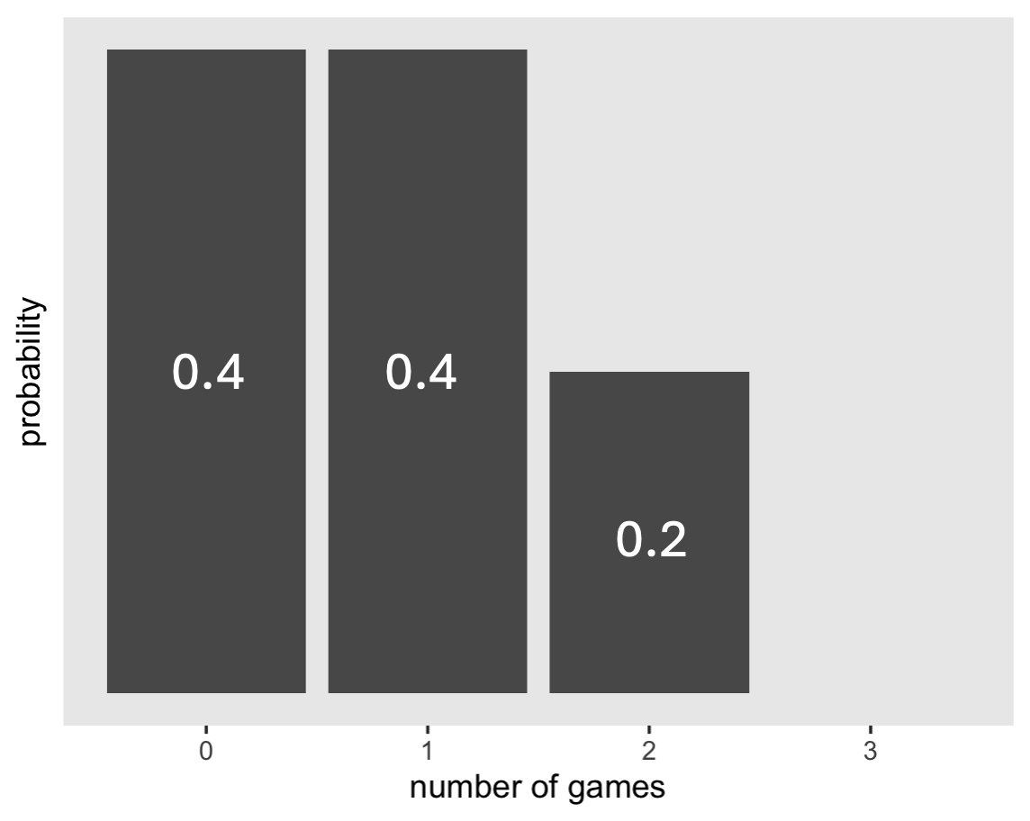
Fig. 2 STAT MS

For reference, the PMF values are tabulated below for accessibility.

Table 6 PMF — STAT HS

Number of games, \(n_g\)	\(P(N_G = n_g \mid \text{STAT HS})\)
0	0.05
1	0.20
2	0.45
3	0.30

Table 7 PMF — STAT MS

Number of games, \(n_g\)	\(P(N_G = n_g \mid \text{STAT MS})\)
0	0.40
1	0.40
2	0.20
3	0.00

---

Question 3a (6 pts)

Given that STAT HS will hold at least one soccer game this month, what is the probability that it holds exactly three?

Solution

We want \(P(N_G = 3 \mid N_G \geq 1,\;\text{STAT HS})\). Writing this out fully using the definition of conditional probability:

\[\begin{split}P(N_G = 3 \mid N_G \geq 1,\;\text{STAT HS}) &= \frac{P(\{N_G = 3\} \cap \{N_G \geq 1\} \cap \{\text{STAT HS}\})}{P(\{N_G \geq 1\} \cap \{\text{STAT HS}\})} \\[6pt] &= \frac{P(N_G = 3 \mid \text{STAT HS})\,P(\text{STAT HS})}{P(N_G \geq 1 \mid \text{STAT HS})\,P(\text{STAT HS})}.\end{split}\]

The factor \(P(\text{STAT HS}) = 0.74\) appears in both numerator and denominator and cancels, leaving:

\[P(N_G = 3 \mid N_G \geq 1,\;\text{STAT HS}) = \frac{P(N_G = 3 \mid \text{STAT HS})}{P(N_G \geq 1 \mid \text{STAT HS})}.\]

Numerator:

\[P(N_G = 3 \mid \text{STAT HS}) = 0.30.\]

Denominator:

\[P(N_G \geq 1 \mid \text{STAT HS}) = 1 - P(N_G = 0 \mid \text{STAT HS}) = 1 - 0.05 = 0.95.\]

Result:

\[P(N_G = 3 \mid N_G \geq 1,\;\text{STAT HS}) = \frac{0.30}{0.95} = \boxed{0.3158}.\]

---

Question 3b (6 pts)

On any given month, what is the probability that at least one game is played?

Solution

Apply the Law of Total Probability, partitioning on the reservation holder:

\[P(N_G \geq 1) = P(N_G \geq 1 \mid \text{STAT HS})\,P(\text{STAT HS}) + P(N_G \geq 1 \mid \text{STAT MS})\,P(\text{STAT MS}).\]

\[P(N_G \geq 1 \mid \text{STAT HS}) = 1 - 0.05 = 0.95, \qquad P(N_G \geq 1 \mid \text{STAT MS}) = 1 - 0.40 = 0.60.\]

\[P(N_G \geq 1) = 0.95 \times 0.74 + 0.60 \times 0.26 = 0.7030 + 0.1560 = \boxed{0.8590}.\]

---

Question 3c (8 pts)

Knowing that at least one game is held next month, what is the probability that the reservation is held by STAT MS?

Solution

Apply Bayes’ Theorem:

\[P(\text{STAT MS} \mid N_G \geq 1) = \frac{P(N_G \geq 1 \mid \text{STAT MS})\,P(\text{STAT MS})}{P(N_G \geq 1)}.\]

Numerator:

\[0.60 \times 0.26 = 0.1560.\]

Denominator (from 3b):

\[P(N_G \geq 1) = 0.8590.\]

Result:

\[P(\text{STAT MS} \mid N_G \geq 1) = \frac{0.1560}{0.8590} = \boxed{0.1816}.\]

---

Question 3d (6 pts)

Are the reservation holder and the number of games played in a month independent? Justify your conclusion mathematically.

Solution

No — they are not independent.

From Question 3c:

\[P(\text{STAT MS} \mid N_G \geq 1) = 0.1816 \neq 0.26 = P(\text{STAT MS}).\]

Since knowing that at least one game was played changes the probability of STAT MS holding the reservation, the two are not independent.

Alternative (more direct) argument: From the PMF, \(P(N_G = 3 \mid \text{STAT MS}) = 0.00\), so if STAT MS holds the reservation, we know for a fact that 3 games will not be played. Therefore the number of games played is not independent of who holds the reservation.

---

Problem 4 (26 points)

Problem 4 Setup

A zombie enthusiast is studying the walking speeds of classic zombies. Based on extensive observations, the enthusiast concludes that the speed of a classic zombie follows a normal distribution with:

• Mean \(\mu = 2\) miles per hour (mph)

• Standard Deviation \(\sigma = 0.19\) mph

Use this information to address the following questions.

---

Question 4a (4 pts)

What is the probability that a randomly chosen classic zombie walks faster than 2.3 mph?

Solution

Let \(F \sim N(\mu = 2,\;\sigma = 0.19)\). Standardize:

\[P(F > 2.3) = P\!\left(Z > \frac{2.3 - 2}{0.19}\right) = P(Z > 1.58) = 1 - \Phi(1.58) = 1 - 0.9429 = \boxed{0.0571}.\]

---

Question 4b (6 pts)

Given that a randomly chosen classic zombie walks faster than 2 mph, what is the probability that it also walks faster than 2.3 mph?

Solution

Since \(\{F > 2.3\} \subset \{F > 2\}\):

\[P(F > 2.3 \mid F > 2) = \frac{P(F > 2.3)}{P(F > 2)}.\]

Numerator (from 4a): \(P(F > 2.3) = 0.0571\).

Denominator: Because \(\mu = 2\), \(P(F > 2) = P(Z > 0) = 0.5000\).

\[P(F > 2.3 \mid F > 2) = \frac{0.0571}{0.5000} = \boxed{0.1142}.\]

---

Question 4c (6 pts)

If the enthusiast randomly selects 10 classic zombies, what is the probability that at least one has a speed greater than 2.3 mph?

Solution

Let \(F_i \overset{\text{iid}}{\sim} N(2,\;0.19)\) for \(i = 1, \ldots, 10\). Use the complement rule — it is much easier to compute the probability that none of the 10 zombies exceed 2.3 mph:

\[\begin{split}P\!\left(\bigcup_{i=1}^{10}\{F_i > 2.3\}\right) &= 1 - P\!\left(\bigcap_{i=1}^{10}\{F_i \leq 2.3\}\right) \\ &= 1 - \prod_{i=1}^{10} P(F_i \leq 2.3) \\ &= 1 - [P(F \leq 2.3)]^{10} \\ &= 1 - (1 - 0.0571)^{10} \\ &= 1 - (0.9429)^{10} \\ &= 1 - 0.5555 = \boxed{0.4445}.\end{split}\]

Complement is key

Computing “at least one” directly would require summing \(P(\text{exactly } k \text{ exceed } 2.3)\) for \(k = 1, 2, \ldots, 10\) — ten separate binomial terms. The complement collapses this to a single calculation.

---

Question 4d (4 pts)

Suppose two classic zombies both begin traveling at the same time. After 3 hours, what is the expected total distance they will have covered combined?

Solution

Since both classic zombies follow the same distribution with expected walking speed \(E[F] = \mu = 2\) mph, and they both walk for 3 hours, each zombie will have covered an expected distance of:

\[E[\text{distance per zombie}] = E[F] \times 3\;\text{hours} = 2 \times 3 = 6\;\text{miles}.\]

By linearity of expectation, the expected combined distance is:

\[E[D_1 + D_2] = E[D_1] + E[D_2] = 6 + 6 = \boxed{12\;\text{miles}}.\]

Note that linearity of expectation holds regardless of whether \(D_1\) and \(D_2\) are independent — it is a universal property of expectation.

---

Question 4e (6 pts)

A classic zombie is considered Elite if its speed is in the top 3%. Determine the minimum speed at which a classic zombie is classified as Elite.

Solution

“Top 3%” means \(P(F \leq f^*) = 0.97\).

Step 1: From the z-table, \(z_{0.97} \approx 1.88\) (since \(\Phi(1.88) = 0.9699 \approx 0.97\)).

Step 2: Transform back:

\[f^* = \mu + z_{0.97} \cdot \sigma = 2 + 1.88 \times 0.19 = 2 + 0.3572 = \boxed{2.3572 \text{ mph}}.\]

---

Problem 5 (26 points)

Problem 5 Setup

At a busy taco truck, customers wait different amounts of time depending on order complexity and queue length. Let \(X\) be the total time, in minutes, from joining the line to receiving food.

No one is served in less than five minutes. The likelihood of finishing follows a parabolic pattern between five and seven and a half minutes, increasing until it peaks at seven and a half. After that, the rate of completion remains constant until twelve and a half minutes, when all orders are fulfilled.

The proposed probability density function has the form

\[\begin{split}f_X(x) = \begin{cases} k\,\bigl(6.25 - (x - 7.5)^2\bigr) & 5 \leq x < 7.5 \\[4pt] \dfrac{25}{4}\,k & 7.5 \leq x < 12.5 \\[4pt] 0 & \text{otherwise} \end{cases}\end{split}\]

where \(k\) must be determined so that \(f_X(x)\) is a valid probability density function.

---

Question 5a (18 pts)

Determine the value of \(k\) such that the function \(f_X(x)\) is a valid PDF.

Solution

A valid PDF must integrate to 1:

\[\int_5^{7.5} k\,(6.25-(x-7.5)^2)\,dx + \int_{7.5}^{12.5} \frac{25}{4}\,k\,dx = 1.\]

Region 2 (constant piece):

\[\int_{7.5}^{12.5} \frac{25}{4}\,k\,dx = \frac{25}{4}\,k \cdot 5 = \frac{125}{4}\,k.\]

Region 1 — substitute \(u = x - 7.5\):

\[k\int_{-2.5}^{0}(6.25 - u^2)\,du = k\!\left[6.25u - \frac{u^3}{3}\right]_{-2.5}^{0} = k\!\left[0 - \left(-15.625 + \frac{15.625}{3}\right)\right] = \frac{125}{12}\,k.\]

Setting the total equal to 1:

\[\frac{125}{12}\,k + \frac{125}{4}\,k = \frac{125 + 375}{12}\,k = \frac{500}{12}\,k = 1 \implies k = \frac{12}{500} = \frac{3}{125} = \boxed{0.0240}.\]

Verification: Region 1 area \(= \tfrac{125}{12} \cdot \tfrac{3}{125} = 0.25\); Region 2 area \(= \tfrac{125}{4} \cdot \tfrac{3}{125} = 0.75\). Total = 1. ✓

---

The cumulative distribution function for the total time, in minutes, from joining the line to receiving food is given by:

\[\begin{split}F_X(x) = \begin{cases} 0 & x < 5 \\[4pt] -\dfrac{1}{125}(x-7.5)^3 + \dfrac{3}{20}\,x - \dfrac{7}{8} & 5 \leq x < 7.5 \\[4pt] \dfrac{3}{20}\,x - \dfrac{7}{8} & 7.5 \leq x < 12.5 \\[4pt] 1 & x \geq 12.5 \end{cases}\end{split}\]

---

Question 5b (8 pts)

The taco truck owner wants to know how long a typical customer waits before receiving their order. Instead of looking at the average, they are interested in the median wait time, the time by which half of all customers have received their food.

Determine the median wait time \(\tilde{\mu}\), where \(P(X \leq \tilde{\mu}) = 0.5\).

Solution

Step 1: Determine which piece of the CDF contains the median.

From the work in part (a), Region 1 (\(5 \leq x < 7.5\)) accumulates a total area of

\[\frac{125}{12}\,k = \frac{125}{12} \times \frac{3}{125} = \frac{1}{4} = 0.25.\]

We can confirm this by evaluating \(F_X(7.5)\):

\[F_X(7.5) = -\frac{1}{125}(0)^3 + \frac{3}{20}(7.5) - \frac{7}{8} = 0 + 1.125 - 0.875 = 0.25.\]

Since \(F_X(7.5) = 0.25 < 0.50\), the 50th percentile (median) must occur in Region 2 (\(7.5 \leq x < 12.5\)), where \(F_X(x) = \dfrac{3}{20}\,x - \dfrac{7}{8}\).

Step 2: Solve \(F_X(\tilde{\mu}) = 0.50\):

\[\frac{3}{20}\,\tilde{\mu} - \frac{7}{8} = \frac{1}{2} \implies \frac{3}{20}\,\tilde{\mu} = \frac{11}{8} \implies \tilde{\mu} = \frac{11}{8} \times \frac{20}{3} = \frac{55}{6} \approx \boxed{9.1667 \text{ minutes}}.\]

Sanity check: The constant density in Region 2 is \(0.15\). Area from 7.5 to 9.1667 under this density: \(0.15 \times 1.6\overline{6} = 0.25\). Adding the 0.25 from Region 1 gives a total of 0.50. ✓