STAT 350 — Exam 1 — Fall 2024
Exam Information
Problem |
Total Possible |
Topic |
|---|---|---|
Problem 1 (True/False, 2 pts each) |
12 |
Data Types, Sampling, Poisson, CDF, z-Scores, Normal |
Problem 2 (Multiple Choice, 3 pts each) |
15 |
Probability, Random Variables, Distributions |
Problem 3 |
20 |
Normal Distribution |
Problem 4 |
26 |
Discrete Probability, Classification |
Problem 5 |
32 |
Piecewise PDF, CDF, Expected Value |
Total |
105 |
The questions below reproduce the Fall 2024 Exam 1 in full accessible text. Each problem is followed by a complete worked solution. Point values reflect the actual exam.
Problem 1: True/False (12 points, 2 points each)
Indicate the correct answer by completely filling in the appropriate circle. If you indicate your answer by any other way, you may be marked incorrect.
Question 1.1 (2 pts)
Employees in a certain UPS branch collected the types of mail customers brought for a month. They plan to present the data appropriately to the manager and discuss how to utilize empty space efficiently.
T or F: A histogram is appropriate to use because the variable is categorical.
Solution
Answer: FALSE
The variable “type of mail” is categorical (qualitative). Histograms are designed for quantitative (numerical) data — they display the distribution of a numerical variable by grouping values into bins. For categorical data, the appropriate displays are bar charts or pie charts, which show frequencies or proportions for each category. The statement is FALSE.
Question 1.2 (2 pts)
A hardware manufacturer is about to ship 20,000 of its products to a client. To estimate the defect rate of this shipment, they randomly selected 100 products for a last-minute inspection. For each product, they assign a value of 0 if the product is good and 1 if it is defective. The defect rate is then calculated as the average of these 0’s and 1’s.
T or F: If the company had the resources to inspect all 20,000 products, the defect rate calculated using all 20,000 products would represent a sample statistic.
Solution
Answer: FALSE
If all 20,000 products in the shipment were inspected, the defect rate would be computed from the entire population of interest (the shipment). A quantity computed from the entire population is a population parameter, not a sample statistic. A sample statistic is computed from a subset (sample) of the population. The statement is FALSE.
Question 1.3 (2 pts)
Suppose the number of visitors to a mall follows a Poisson distribution with an average rate of 45 visitors per 30 minutes.
T or F: In this mall, the variance in the number of visitors arriving between 2:00 PM and 3:00 PM is equal to the variance in the number of visitors arriving between 3:00 PM and 5:00 PM.
Solution
Answer: FALSE
For a Poisson process with rate \(\lambda\) visitors per 30 minutes, the number of visitors in a time interval of length \(t\) (in 30-minute units) follows \(\text{Poisson}(\lambda t)\), which has variance \(\lambda t\).
2:00 PM to 3:00 PM is 1 hour = 2 thirty-minute periods: \(\text{Var} = 45 \times 2 = 90\) visitors².
3:00 PM to 5:00 PM is 2 hours = 4 thirty-minute periods: \(\text{Var} = 45 \times 4 = 180\) visitors².
The variances are not equal. The statement is FALSE.
Question 1.4 (2 pts)
Let \(V\) be a random variable with a probability density function \(f_V(v)\) that is nonzero only on the interval \([-5, -2)\). Let \(F_V(\cdot)\) denote the cumulative distribution function (CDF) of \(V\).
T or F: Then, \(F_V(c) = 1\) holds for any \(c > 0\).
Solution
Answer: TRUE
The support of \(V\) is entirely contained in \([-5, -2)\). For any \(c > 0\), since \(0 > -2\), the value \(c\) lies strictly to the right of the entire support. The CDF at \(c\) accumulates all probability mass in \((-\infty, c]\), which includes the entire support \([-5, -2)\). Therefore \(F_V(c) = 1\) for all \(c > 0\). The statement is TRUE.
Question 1.5 (2 pts)
A student scored 85 on two different math exams. For Exam 1, the mean score is 75 with a standard deviation of 5, and for Exam 2, the mean score is 70 with a standard deviation of 10.
T or F: The student performed better on Exam 1 compared to Exam 2.
Solution
Answer: TRUE
Compute the z-score for each exam to compare relative performance:
Since \(z_{\text{Exam 1}} = 2.00 > 1.50 = z_{\text{Exam 2}}\), the student scored 2 standard deviations above the mean on Exam 1 but only 1.5 standard deviations above the mean on Exam 2. The student performed relatively better on Exam 1. The statement is TRUE.
Question 1.6 (2 pts)
For the figure below,
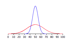
T or F: the blue normal distribution has more area underneath its curve than the red normal distribution does.
Solution
Answer: FALSE
Every normal distribution, regardless of its mean \(\mu\) or standard deviation \(\sigma\), has total area equal to 1 under its curve. This is a fundamental property of all probability density functions. The blue curve is taller and narrower (smaller \(\sigma\)) while the red curve is shorter and wider (larger \(\sigma\)), but both enclose exactly the same total area of 1. The statement is FALSE.
Problem 2: Multiple Choice (15 points, 3 points each)
Indicate the correct answer by completely filling in the appropriate circle. If you indicate your answer by any other way, you may be marked incorrect. For each question, there is only one correct option letter choice.
Question 2.1 (3 pts)
The number of customers arriving at a UPS branch during working hours follows a Poisson distribution with an average rate of 4 customers per hour. Let \(X\) denote the number of customers arriving between 9:00 AM and 10:00 AM and let \(Y\) denote the number of customers arriving between 10:30 AM and 12:00 PM.
What is the conditional probability that exactly 3 customers arrive between 10:30 AM and 12:00 PM, given that 6 customers arrived between 9:00 AM and 10:00 AM?
(A) \(P(Y = 3 \mid X = 6) = 0\)
(B) \(P(Y = 3 \mid X = 6) = 0.0093\)
(C) \(P(Y = 3 \mid X = 6) = 0.0892\)
(D) \(P(Y = 3 \mid X = 6) = 0.1954\)
(E) \(P(Y = 3 \mid X = 6) = 0.8564\)
Solution
Answer: (C)
The intervals 9:00–10:00 AM and 10:30 AM–12:00 PM do not overlap. For a Poisson process, arrivals in non-overlapping intervals are independent. Therefore:
The interval 10:30 AM–12:00 PM is 1.5 hours long. With a rate of 4 customers per hour:
The answer is (C).
Question 2.2 (3 pts)
The time between customer arrivals at the same UPS facility follows an exponential distribution with an average of 15 minutes between customer arrivals. Let \(T\) denote the time between customer arrivals. If no customer has arrived in the last 20 minutes, what is the probability that the next customer arrives after waiting more than 15 additional minutes.
(A) \(P(T > 35 \mid T > 20) = 0\)
(B) \(P(T > 35 \mid T > 20) = 0.097\)
(C) \(P(T > 35 \mid T > 20) = 0.2636\)
(D) \(P(T > 35 \mid T > 20) = 0.3679\)
(E) \(P(T > 35 \mid T > 20) = 0.6321\)
Solution
Answer: (D)
The Exponential distribution has the memoryless property:
Applying this with \(s = 20\) and \(t = 15\):
Since \(T \sim \text{Exponential}\!\left(\lambda = \dfrac{1}{15}\right)\):
The answer is (D).
Question 2.3 (3 pts)
Suppose \(X \sim \text{Binomial}(n = 10,\; p = 0.1)\) and \(Y \sim \text{Binomial}(n = 10,\; p = 0.9)\).
Which statement is not always true about \(X\) and \(Y\)?
(A) The mode of \(X\) is less than the mode of \(Y\).
(B) \(\text{SD}(X) - |\sqrt{\text{Var}(Y)}| = 0\)
(C) \(P(X = 1 \cap Y = 8) = 0.1943\)
(D) \(E[X^2] = (10)(0.1)(0.9) + [(10)(0.1)]^2\)
(E) \(P(X = 1) = P(Y = 9)\)
Solution
Answer: (A)
Evaluate each option:
(A) For \(X \sim \text{Bin}(10, 0.1)\), the mode is \(\lfloor(n+1)p\rfloor = \lfloor 1.1 \rfloor = 1\). For \(Y \sim \text{Bin}(10, 0.9)\), the mode is \(\lfloor(n+1)(0.9)\rfloor = \lfloor 9.9 \rfloor = 9\). The mode of \(X\) is 1 and the mode of \(Y\) is 9, and \(1 < 9\). While this appears true for these specific distributions, the Binomial mode is not always strictly less than or greater than another Binomial mode in general — it depends on the specific parameters and whether modes are unique.
(B) Always true. \(\text{SD}(X) = \sqrt{np(1-p)} = \sqrt{10(0.1)(0.9)} = \sqrt{0.9}\). Similarly \(\sqrt{\text{Var}(Y)} = \sqrt{10(0.9)(0.1)} = \sqrt{0.9}\). Their difference is 0.
(C) Never true. If \(X\) and \(Y\) are independent, \(P(X=1 \cap Y=8) = P(X=1) \cdot P(Y=8) \approx 0.3874 \times 0.1937 \approx 0.0750 \neq 0.1943\).
(D) Always true. Using \(E[X^2] = \text{Var}(X) + (E[X])^2 = np(1-p) + (np)^2 = (10)(0.1)(0.9) + [(10)(0.1)]^2\).
(E) Always true. By symmetry of the Binomial: \(P(X = k) = P(Y = n-k)\), so \(P(X=1) = P(Y=9)\).
The answer is (A).
Question 2.4 (3 pts)
Suppose \(X\) is a random variable with \(E[e^X] = 2\) and \(\text{Var}(e^X) = 5\), and \(Y\) is a random variable independent of \(X\), satisfying \(E(Y) = -10\), \(\text{Var}(Y) = 3\). What is \(E\!\left[(e^X - 3Y)^2\right]\)?
(A) 1056
(B) 240
(C) 1024
(D) -752
(E) None of the above
Solution
Answer: (A)
Expand the square:
Find each term:
\(E[e^{2X}]\): using \(\text{Var}(e^X) = E[e^{2X}] - (E[e^X])^2\):
\(E[e^X Y]\): since \(X\) and \(Y\) are independent:
\(E[Y^2]\): using \(\text{Var}(Y) = E[Y^2] - (E[Y])^2\):
Combine:
The answer is (A).
Question 2.5 (3 pts)
The figure below shows the shape of the distribution for two continuous random variables \(X\) and \(Y\).
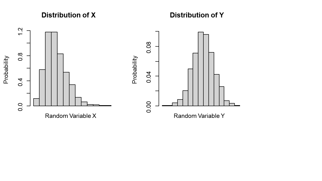
Which of the following statements is TRUE about the random variable \(X\)?
(A) The mean is a better measure of central tendency than median.
(B) The distance between \(Q_3\) and the median is narrower than the distance between \(Q_1\) and the median.
(C) IQR is a robust (resistant) measure of the spread.
(D) The distribution is negatively skewed with one peak.
(E) The mode will have the largest value among all the measures of central tendency.
Solution
Answer: (C)
The distribution of \(X\) is right-skewed (positively skewed) with a long right tail. Evaluate each option:
(A) FALSE. For a right-skewed distribution, the mean is pulled toward the long right tail and is not resistant to extreme values. The median is a better (more resistant) measure of central tendency than the mean for skewed data.
(B) FALSE. For a right-skewed distribution, the bulk of the data is concentrated on the left, so the right half of the box (Q₃ to median) is typically wider than the left half (Q₁ to median). The distance from \(Q_3\) to the median is not narrower.
(C) TRUE. The IQR is based on the middle 50% of the data and is not affected by extreme values or outliers in the tails. It is a robust (resistant) measure of spread, regardless of the shape of the distribution.
(D) FALSE. The histogram of \(X\) shows a right tail (positively skewed), not negatively skewed.
(E) FALSE. For a right-skewed distribution, the ordering of measures of central tendency is Mode < Median < Mean. The mode has the smallest value, not the largest.
The answer is (C).
Free Response Questions 3–5
Show all work, clearly label your answers, and use four decimal places.
Problem 3 (20 points)
Problem 3 Setup
The stated speed limit on I-65 is 65 mph. The speeds of vehicles along a certain stretch of I-65 follow an approximately normal distribution with a mean of 71 mph and a standard deviation of 8 mph.
Let \(V\) denote the speed of a random vehicle on I-65.
Question 3a (2 pts)
What is the probability that the speed of a vehicle on this stretch of I-65 is below \(\mu + 3\sigma\)?
Solution
Simply using the Empirical Rule:
Question 3b (2 pts)
Calculate the z-score for the stated speed limit of 65 mph.
Solution
Question 3c (8 pts)
What is the probability that a vehicle’s speed is between 61 mph and 71 mph on this stretch of I-65?
Solution
Using the z-table and symmetry:
Question 3d (8 pts)
State patrol officers will issue radar tickets to vehicles whose speeds are in the top 4% of this distribution. What is the speed cutoff for issuing tickets?
Solution
The top 4% corresponds to the 96th percentile.
From the z-table: \(\Phi(1.75) = 0.9599 \approx 0.96\), so \(z = 1.75\).
Transform to the distribution of car speeds on I-65:
The cutoff for the top 4% of vehicle speeds on I-65 is 85 miles per hour.
Problem 4 (26 points)
Problem 4 Setup
Kristin, a data science major, is working on a term project to build a predictive model that can classify images of handwritten digits (0–4).
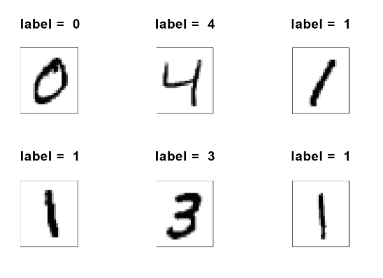
She has a dataset containing 1600 images, each displaying a single digit. Kristin divided the dataset into a training set of 1000 images and a test set of 600 images. The training set is used to teach the model, while the test set is used to evaluate its performance.
After training, Kristin used the test set to create a confusion matrix, which shows the number of correctly and incorrectly classified images. In the matrix below, rows indicate the actual labels (ground truth), and columns represent the predicted labels made by the model:
True Label |
Predicted Label |
||||||
|---|---|---|---|---|---|---|---|
Digits |
0 |
1 |
2 |
3 |
4 |
Total |
|
0 |
107 |
0 |
0 |
1 |
8 |
116 |
|
1 |
0 |
117 |
1 |
0 |
4 |
122 |
|
2 |
0 |
4 |
92 |
11 |
1 |
108 |
|
3 |
3 |
1 |
15 |
112 |
1 |
132 |
|
4 |
4 |
0 |
0 |
4 |
114 |
122 |
|
Total |
114 |
122 |
108 |
128 |
128 |
600 |
|
Reading the Table: The highlighted cell with the value 117 indicates that the model correctly predicted the digit ‘1’ for 117 images that had True Label as ‘1’. This number represents the model’s accurate classifications for the digit ‘1’ in the test set.
All questions below refer to the data presented in the confusion matrix (table).
Question 4a (3 pts)
Define the events:
\(E_1 = \{\text{true label is 4}\}\)
\(E_2 = \{\text{true label is 1 or 2}\}\)
\(E_3 = \{\text{predicted label is 0}\}\)
Which of the following statements is TRUE?
(A) Two events \(E_1\) and \(E_3\) are mutually exclusive.
(B) \(P(E_1 \cap E_3) = P(E_1)\,P(E_3)\).
(C) Two events \(E_1\) and \(E_2\) are disjoint.
(D) \(P(E_2 \cup E_3) > P(E_2) + P(E_3)\).
Solution
Answer: (C)
Check each statement using the confusion matrix:
(A) FALSE. \(E_1 \cap E_3\) = {true label is 4 AND predicted label is 0}. From the matrix, 4 images have true label 4 and were predicted as 0. So \(P(E_1 \cap E_3) = 4/600 \neq 0\). They are not mutually exclusive.
(B) FALSE. \(P(E_1) = 122/600\), \(P(E_3) = 114/600\), \(P(E_1 \cap E_3) = 4/600\). Check: \(P(E_1)P(E_3) = (122/600)(114/600) = 13908/360000 \approx 0.0386\), but \(P(E_1 \cap E_3) = 4/600 \approx 0.0067\). Not equal.
(C) TRUE. \(E_1\) = {true label is 4} and \(E_2\) = {true label is 1 or 2}. An image cannot simultaneously have true label 4 and true label 1 or 2. Therefore \(E_1 \cap E_2 = \emptyset\) and the events are disjoint.
(D) FALSE. By the inclusion-exclusion principle: \(P(E_2 \cup E_3) = P(E_2) + P(E_3) - P(E_2 \cap E_3)\). Since \(P(E_2 \cap E_3) \geq 0\), we always have \(P(E_2 \cup E_3) \leq P(E_2) + P(E_3)\).
The following events are used in Questions 4b–4e. Kristin wants to know if the model performs better than random guessing at classifying images of the digit three.
\(T_3 = \{\text{true label is 3}\}\)
\(P_3 = \{\text{predicted label is 3}\}\)
Question 4b (5 pts)
What is the probability that a randomly selected image has the true label three?
Solution
From the Total row, 132 images have true label 3 out of 600 total:
Question 4c (5 pts)
What is the probability that a randomly selected image is predicted to be three?
Solution
From the Total column, 128 images were predicted as 3 out of 600 total:
Question 4d (8 pts)
What is the probability that an image of digit three is correctly predicted to be three?
Solution
This is the conditional probability \(P(P_3 \mid T_3)\). Of the 132 images with true label 3, the model correctly predicted 112 as 3:
Question 4e (5 pts)
Are the events \(T_3\) and \(P_3\) independent? State your answer and provide a mathematical justification.
Solution
No, they are not independent, as the conditional probability does not equal the unconditional probability:
Since \(P(P_3 \mid T_3) \neq P(P_3)\), the events \(T_3\) and \(P_3\) are not independent.
Problem 5 (32 points)
Problem 5 Setup
Robust-ish Devices Inc. manufactures devices whose lifetimes are divided into three distinct phases: early failure, stable operation, and wear-out.
Phase 1 (Early Failure): During the first year (\(0 \leq x \leq 1\)), the device has a constant likelihood of failing due to manufacturing defects, meaning the probability density function (pdf) for the device’s lifetime is constant in this interval.
Phase 2 (Stable Operation): After surviving the early failure phase, the device operates reliably with virtually no chance of failure for the next 4 years (\(1 < x \leq 5\)), meaning the pdf is zero during this phase, as the device is highly reliable.
Phase 3 (Wear Out): Beyond 5 years (\(x > 5\)), the device enters a wear-out phase where the likelihood of failure increases over time. The lifetime is modeled by an exponentially decaying function, meaning the chance of the device surviving much longer decreases, and the risk of failure increases as the device ages.
The probability density function for \(X\) (the lifetime of the device) is given by the following piecewise function:
Question 5a (10 pts)
Verify that \(f_X(x)\) is a valid probability density function.
Solution
Axiom 1: \(f_X(x) \geq 0\) clearly by the graph of the pdf or because it is a positive constant over \(0 \leq x \leq 1\), an exponentially decaying function over \(x \geq 5\), and 0 everywhere else.
Axiom 2:
The cumulative distribution function is partially given below:
Question 5b (10 pts)
Determine the missing value of the cumulative distribution function (CDF) \(F_X(x)\), which is partially given above.
Solution
For \(x \geq 5\), integrate from 5 to \(x\) and add the accumulated area through the stable phase:
Question 5c (4 pts)
Determine the probability that the device lasts longer than 1 year.
Solution
Question 5d (8 pts)
Find the 25th percentile for the lifetime of devices manufactured by Robust-ish Devices Inc..
Solution
The 25th percentile \(x^*\) satisfies \(F_X(x^*) = 0.25\).
First determine which region contains \(x^*\). The CDF reaches \(F_X(1) = 1 - e^{-5/16} \approx 0.2684\) at \(x = 1\), and remains at 0.2684 until \(x = 5\). Since \(0.25 < 0.2684\), the 25th percentile falls in the region \([0, 1)\).
Solve \(F_X(x^*) = 0.25\) for the region \([0, 1)\):
The 25th percentile of lifetime is 0.9315 years.