Exam 1 — Spring 2024: Fully Worked Solutions

• Exam PDF

• Solution PDF

The questions below reproduce the Spring 2024 Exam 1 in full accessible text. Each problem is followed by a complete worked solution. Point values reflect the actual exam.

Table 3 Point Summary

Section	Format	Points
Problem 1 — True/False	6 questions × 2 pts	12
Problem 2 — Multiple Choice	5 questions × 3 pts	15
Problem 3 — Free Response	4 parts	24
Problem 4 — Free Response	3 parts	24
Problem 5 — Free Response	5 parts	30
Total		105

---

Problem 1: True/False (12 points, 2 points each)

Indicate the correct answer by completely filling in the appropriate circle. If you indicate your answer by any other way, you may be marked incorrect.

---

Question 1.1 (2 pts)

Let \(X \sim \text{Binomial}(n, p = 0.5)\), where \(n\) is any positive integer.

T or F: For any value of \(x\) in the support of \(X\), \(P(X = x) = P(X = n - x)\).

Solution

Answer: TRUE

For \(X \sim \text{Binomial}(n, p)\), the PMF is \(P(X = x) = \binom{n}{x} p^x (1-p)^{n-x}\).

With \(p = 0.5\):

\[P(X = x) = \binom{n}{x} (0.5)^x (0.5)^{n-x} = \binom{n}{x} (0.5)^n.\]

\[P(X = n-x) = \binom{n}{n-x} (0.5)^{n-x} (0.5)^{x} = \binom{n}{n-x} (0.5)^n.\]

Since \(\dbinom{n}{x} = \dbinom{n}{n-x}\), we have \(P(X=x) = P(X=n-x)\). The statement is TRUE.

---

Question 1.2 (2 pts)

Suppose two events \(A\) and \(B\) are in the sample space \(\Omega\) with all outcomes of \(A\) contained within the event \(B\).

T or F: In this scenario it must follow that \(P(A \cap B) = P(B)\).

Solution

Answer: FALSE

If all outcomes of \(A\) are contained within \(B\), then \(A \subseteq B\), which means \(A \cap B = A\). Therefore:

\[P(A \cap B) = P(A).\]

The statement claims \(P(A \cap B) = P(B)\), which would require \(P(A) = P(B)\). This is not necessarily true — \(A\) can be a proper subset of \(B\) with \(P(A) < P(B)\). The statement is FALSE.

---

Question 1.3 (2 pts)

Given two non-empty events \(A\) and \(B\) of a sample space \(\Omega\),

T or F: if \(P(A \mid B) = P(A)\) then we are certain that \(A \cap B \neq \emptyset\).

Solution

Answer: TRUE

Since \(A\) and \(B\) are non-empty events, \(P(A) > 0\) and \(P(B) > 0\).

From the definition of conditional probability:

\[P(A \mid B) = \frac{P(A \cap B)}{P(B)} = P(A) \implies P(A \cap B) = P(A) \cdot P(B).\]

Since \(P(A) > 0\) and \(P(B) > 0\):

\[P(A \cap B) = P(A) \cdot P(B) > 0.\]

A positive probability means the event \(A \cap B\) cannot be empty. The statement is TRUE.

---

Question 1.4 (2 pts)

Let \(X\) be a random variable that satisfies the conditions to be distributed as Poisson.

T or F: The expected value must satisfy \(E[X] > 0\).

Solution

Answer: TRUE

For a Poisson distribution, the parameter \(\lambda\) represents the average rate of events and must satisfy \(\lambda > 0\). Since \(E[X] = \lambda\), it follows directly that \(E[X] = \lambda > 0\). The statement is TRUE.

---

Question 1.5 (2 pts)

Given a five number summary for a dataset we could compute the interquartile range, identify the fences, and draw a modified box plot to visualize properties of the data.

T or F: The upper whisker of the modified boxplot would be drawn to terminate at the point \(Q_3 + 1.5 \times IQR\).

Solution

Answer: FALSE

The upper inner fence is located at \(Q_3 + 1.5 \times IQR\), but the upper whisker does not necessarily terminate there. The upper whisker is drawn to the largest observed data value that falls at or below the upper inner fence. If the maximum non-outlier value is less than \(Q_3 + 1.5 \times IQR\), the whisker terminates before reaching the fence. The statement is FALSE.

---

Question 1.6 (2 pts)

For a random variable \(X\) that follows a normal distribution,

T or F: the mode of \(X\) is always greater than its mean.

Solution

Answer: FALSE

The normal distribution is symmetric and unimodal. Its mean, median, and mode all coincide at \(\mu\). Therefore the mode equals the mean, and it is impossible for the mode to be greater than the mean. The statement is FALSE.

---

Problem 2: Multiple Choice (15 points, 3 points each)

Indicate the correct answer by completely filling in the appropriate circle. If you indicate your answer by any other way, you may be marked incorrect. For each question, there is only one correct option letter choice.

---

Question 2.1 (3 pts)

Let \(X\) be a random variable with mean \(\mu_X = 7\) and standard deviation \(\sigma_X = 9\). Define another random variable \(Y = 2X^2 + 5X + 3\). Determine the value of \(E[Y]\).

• (A) \(E[Y] = 136\)

• (B) \(E[Y] = 200\)

• (C) \(E[Y] = 214\)

• (D) \(E[Y] = 298\)

• (E) Not enough information to calculate it.

Solution

Answer: (D)

Apply linearity of expectation:

\[E[Y] = E[2X^2 + 5X + 3] = 2\,E[X^2] + 5\,E[X] + 3.\]

Find \(E[X^2]\) using the variance identity \(\text{Var}(X) = E[X^2] - (E[X])^2\):

\[E[X^2] = \text{Var}(X) + (E[X])^2 = \sigma_X^2 + \mu_X^2 = 9^2 + 7^2 = 81 + 49 = 130.\]

Therefore:

\[E[Y] = 2(130) + 5(7) + 3 = 260 + 35 + 3 = \boxed{298}.\]

The answer is (D).

---

Question 2.2 (3 pts)

Identify the false statement regarding a continuous random variable \(Y\), which has support extending from 0 to infinity.

(Note: The pdf and cdf of the random variable \(Y\) is denoted by \(f_Y(y)\) and \(F_Y(y)\) respectively.)

• (A) If \(y_1\) and \(y_2\) are values in the support with \(y_1 < y_2\), then it follows that \(F_Y(y_1) \leq F_Y(y_2)\).

• (B) If \(y\) is a value in the support, \(f_Y(y) > 0\).

• (C) If \(y\) is a value in the support, \(P(Y = y) > 0\).

• (D) It is possible for \(f_Y(y)\) to be a decreasing function for all values of \(y\) in the support.

• (E) If \(y_1\) and \(y_2\) are values in the support with \(y_1 < y_2\), it is possible that \(f_Y(y_1) > f_Y(y_2)\).

Solution

Answer: (C)

(A) TRUE. The CDF is a non-decreasing function by definition.

(B) TRUE. A value in the support of a continuous random variable has positive density by the definition of support.

(C) FALSE. For any continuous random variable, the probability of any single exact value is zero: \(P(Y = y) = 0\) for all \(y\). Probabilities for continuous random variables are only positive over intervals (via integration of the pdf). The statement is FALSE.

(D) TRUE. A decreasing pdf is possible — the Exponential distribution, for example, has \(f(y) = \lambda e^{-\lambda y}\) which is strictly decreasing for all \(y > 0\).

(E) TRUE. The pdf does not need to be monotone; it is possible (and common) for the density to be larger at a smaller value than at a larger value.

---

Question 2.3 (3 pts)

In Cerulean city, 3.2 car accidents are reported on average per day. The number of car accidents is known to follow a Poisson distribution. What is the probability that at least one accident occurs per day? Let \(X\) denote the Poisson random variable for this situation.

• (A) \(P(X \geq 1) = 0.9592\)

• (B) \(P(X \geq 1) = 0.0408\)

• (C) \(P(X \geq 1) = 0.1712\)

• (D) \(P(X \geq 1) = 0.8288\)

• (E) None of the above

Solution

Answer: (A)

Use the complement rule:

\[P(X \geq 1) = 1 - P(X = 0) = 1 - \frac{e^{-3.2} \cdot 3.2^0}{0!} = 1 - e^{-3.2}.\]

\[e^{-3.2} \approx 0.0408,\]

\[P(X \geq 1) = 1 - 0.0408 = \boxed{0.9592}.\]

The answer is (A).

---

Question 2.4 (3 pts)

Suppose a random variable \(X\) follows a normal distribution with an unknown mean \(\mu\) and unknown variance \(\sigma^2\). Then \(P(X > \mu + \sigma)\) is approximately equal to?

• (A) 0.16

• (B) 0

• (C) 0.25

• (D) 0.5

• (E) Not enough information available.

Solution

Answer: (A)

Standardize:

\[P(X > \mu + \sigma) = P\!\left(Z > \frac{(\mu + \sigma) - \mu}{\sigma}\right) = P(Z > 1).\]

From the z-table:

\[P(Z > 1) = 1 - \Phi(1) = 1 - 0.8413 = 0.1587 \approx \boxed{0.16}.\]

This result holds for any normal distribution regardless of the values of \(\mu\) and \(\sigma^2\). The answer is (A).

---

Question 2.5 (3 pts)

At Lumina Tech, a software development company, the project management team conducted an analysis to understand the distribution of time spent on five categories: Quick Fixes, Feature Development, Bug Fixes, Code Review, and Team Meetings. Analyzing monthly data of 32 employees, they generated side-by-side boxplots for each category to illustrate time distributions. Using the side-by-side boxplot approximate the number of employees that spent more than 15 hours on Bug Fixes.

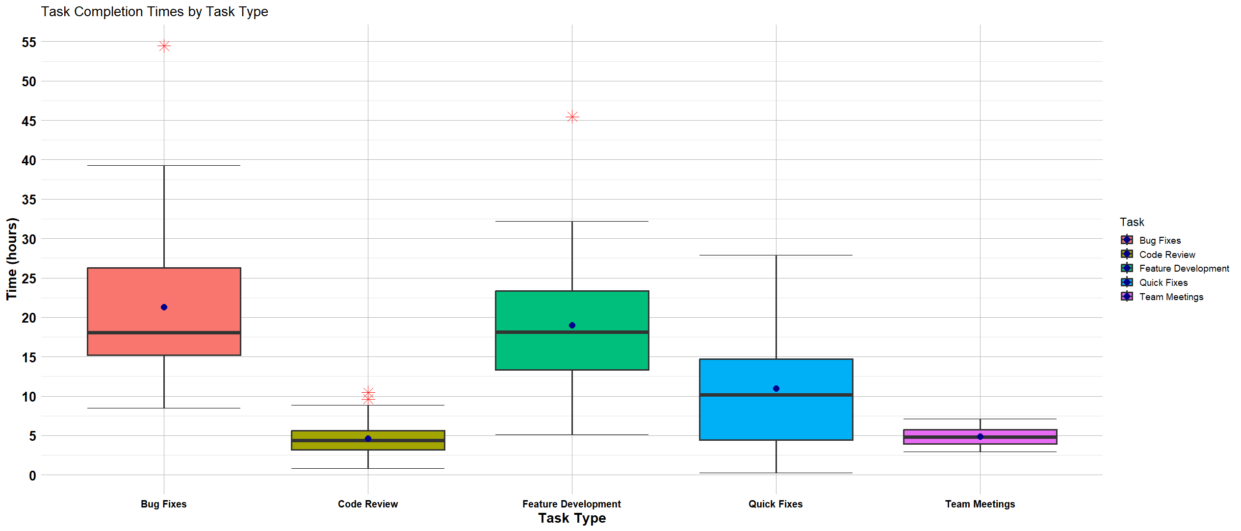
• (A) 8 employees

• (B) 16 employees

• (C) 24 employees

• (D) 30 employees

• (E) Not enough information available.

Solution

Answer: (C)

From the boxplot, the first quartile (\(Q_1\)) of Bug Fixes is approximately 15 hours. By definition, \(Q_1\) is the 25th percentile — meaning 25% of employees spent less than 15 hours and 75% spent more than 15 hours on Bug Fixes.

\[0.75 \times 32 = 24 \text{ employees}.\]

The answer is (C).

---

Free Response Questions 3–5

Show all work, clearly label your answers, and use four decimal places.

Problem 3 (24 points)

Problem 3 Setup

Marina orders her dinner from Doordash. When she places an order, it is known to take 35 minutes on average for delivery. Assume each order’s delivery time is independent of others.

---

Question 3a (4 pts)

Define the continuous random variable \(X\) which represents the amount of time (in minutes) Marina waits for her delivery. Write the name of its distribution and provide the value of the parameter, \(\lambda\) or \(\mu\).

Solution

\[X \sim \text{Exponential}\!\left(\lambda = \frac{1}{35}\right).\]

The pdf is \(f_X(x) = \dfrac{1}{35}\,e^{-x/35}\) for \(x \geq 0\).

---

Question 3b (4 pts)

What is the probability that Marina will wait exactly 38 minutes for her delivery?

Solution

Since \(X\) is a continuous random variable, the probability of any single exact value is zero:

\[P(X = 38) = \boxed{0}.\]

---

Question 3c (6 pts)

What is the probability that Marina will wait more than 25 minutes for her delivery?

Solution

Using the survival function of the Exponential distribution:

\[P(X > 25) = \int_{25}^{\infty} \frac{1}{35}\,e^{-x/35}\,dx = e^{-25/35} = e^{-5/7} \approx \boxed{0.4895}.\]

---

Question 3d (10 pts)

If the delivery takes less than 25 minutes, Marina will add an additional tip to the deliverer. Assume she placed 10 orders in January. What is the probability that Marina adds additional tip for 2 orders out of 10 orders?

Solution

Let \(Y\) denote the number of orders for which Marina adds an additional tip. This is a Binomial random experiment:

\[Y \sim \text{Binomial}\!\left(n = 10,\; p = 1 - e^{-25/35}\right).\]

\[P(Y = 2) = \binom{10}{2}\,(1 - e^{-25/35})^2\,(e^{-25/35})^8 = \boxed{0.0387}.\]

---

Problem 4 (24 points)

Problem 4 Setup

Health authorities at Lumina University observed that the weights of their students follow a normal distribution. Furthermore, their assessment revealed that the mean weight of their students is 160 lbs, with a variance of 25 lbs². Using this information, answer the following questions.

Let \(W\) be defined as the weight of a random student at Lumina University.

\[W \sim \text{Normal}(\mu = 160,\; \sigma^2 = 25), \quad \sigma = 5.\]

---

Question 4a (6 pts)

What is the probability that a student at Lumina University weighs at least 156 lbs?

Solution

Standardize:

\[P(W \geq 156) = P\!\left(Z \geq \frac{156 - 160}{5}\right) = P(Z \geq -0.8).\]

By symmetry of the standard normal:

\[P(Z \geq -0.8) = P(Z \leq 0.8) = \Phi(0.8) = \boxed{0.7881}.\]

---

Question 4b (8 pts)

What is the probability that a student at Lumina University weighs between 160 lbs and 168 lbs?

Solution

\[P(160 < W < 168) = P(W < 168) - P(W < 160).\]

Standardize each:

\[P\!\left(Z < \frac{168 - 160}{5}\right) - P\!\left(Z < \frac{160 - 160}{5}\right) = P(Z < 1.6) - P(Z < 0).\]

From the z-table:

\[= \Phi(1.6) - \Phi(0) = 0.9452 - 0.5000 = \boxed{0.4452}.\]

---

Question 4c (10 pts)

Lumina University’s health officials declared 0.25% of students overweight. What cutoff value was used by them to determine whether a student is overweight or not?

Solution

The upper 0.25% is the same cutoff as the lower 99.75th percentile.

Step 1: Find \(z_{0.9975}\) from the z-table such that \(P(Z < z) = 0.9975\):

\[z_{0.9975} = 2.81 \quad (\text{since } \Phi(2.81) = 0.9975).\]

Step 2: Transform back:

\[w_{0.9975} = \mu + z_{0.9975} \cdot \sigma = 160 + 2.81 \times 5 = 160 + 14.05 = \boxed{174.05 \text{ lbs}}.\]

---

Problem 5 (30 points)

Problem 5 Setup

In a nanotechnology lab, researchers study ultraviolet light’s effect on nanostructures, focusing on wavelengths between 6 and 14 nanometers. The probability density function (PDF) models the distribution of these interactions, aiding in the development of materials with specific optical properties. Before analyzing these interactions, it’s crucial to establish the normalizing constant for precise probability calculations.

\[\begin{split}f_X(x) = \begin{cases} k\,(x - 6) & 6 \leq x \leq 8 \\[4pt] 2k & 8 < x \leq 12 \\[4pt] k\,(14 - x) & 12 < x \leq 14 \\[4pt] 0 & \text{otherwise} \end{cases}\end{split}\]

---

Question 5a (10 pts)

Determine the value of the constant \(k\) such that the function is a valid probability density function.

Solution

First, note \(k > 0\) is required, otherwise \(f_X(x) < 0\) on the support.

Set the total area equal to 1:

\[k \left[\int_6^8 (x-6)\,dx + 2\int_8^{12} dx + \int_{12}^{14}(14-x)\,dx\right] = 1.\]

Using the substitutions \(u = x - 6\) and \(v = 14 - x\):

\[k \left[\int_0^2 u\,du + 2\int_8^{12} dx - \int_2^0 v\,dv\right] = 1.\]

\[k \left[\frac{u^2}{2}\bigg|_0^2 + 2(12-8) + \frac{v^2}{2}\bigg|_0^2\right] = 1.\]

\[k\left[2 + 8 + 2\right] = 1 \implies 12k = 1 \implies k = \boxed{\frac{1}{12}}.\]

---

The cumulative distribution function is:

\[\begin{split}F_X(x) = \begin{cases} [A] & x < 6 \\[4pt] [B] & 6 \leq x < 8 \\[4pt] \dfrac{x - 7}{6} & 8 \leq x < 12 \\[4pt] 1 - \dfrac{(x-14)^2}{24} & 12 \leq x < 14 \\[4pt] [C] & x \geq 14 \end{cases}\end{split}\]

---

Question 5b (6 pts)

Determine the missing parts [A], [B], and [C] for the cumulative distribution function \(F_X(x)\) above.

Solution

[A] — Below the support, no area has accumulated:

\[[A] = \boxed{0}.\]

[C] — Above the support, all area has been accumulated:

\[[C] = \boxed{1}.\]

[B] — Integrate the pdf from 6 to \(x\) for \(6 \leq x < 8\):

\[F_X(x) = \int_6^x \frac{1}{12}(t-6)\,dt = \frac{1}{12}\cdot\frac{(t-6)^2}{2}\bigg|_6^x = \frac{(x-6)^2}{24}.\]

\[[B] = \boxed{\dfrac{(x-6)^2}{24}}.\]

---

Question 5c (6 pts)

Determine the probability that the wavelength of UV light interacting with a nanostructure is between 10 and 12 nanometers.

Solution

Both 10 and 12 fall in the region \(8 \leq x < 12\), where \(F_X(x) = \dfrac{x-7}{6}\):

\[P(10 < X < 12) = F_X(12) - F_X(10) = \frac{12-7}{6} - \frac{10-7}{6} = \frac{5}{6} - \frac{3}{6} = \frac{2}{6} = \frac{1}{3} = \boxed{0.3333}.\]

---

Question 5d (4 pts)

Calculate the mean wavelength (expected value) of UV light interacting with nanostructures.

Solution

The distribution is symmetric about 10 and therefore the mean and median are both 10.

\[E[X] = \boxed{10 \text{ nanometers}}.\]

---

Question 5e (4 pts)

The function \(g(X) = 0.1X - 0.5\) approximates the intensity of light absorption of the nanostructures. Given that the variance of the UV light interacting with the nanostructures is known to be \(\sigma_X^2 = \dfrac{10}{3}\), determine the standard deviation of the intensity of light absorption of the nanostructures.

Solution

Apply the linear transformation rule for variance:

\[\text{Var}(g(X)) = \text{Var}(0.1X - 0.5) = (0.1)^2\,\text{Var}(X) = 0.01 \times \frac{10}{3} = \frac{0.1}{3}.\]

The standard deviation is:

\[\text{SD}(g(X)) = \sqrt{\frac{0.1}{3}} = 0.1\sqrt{\frac{10}{3}} = \boxed{0.1826}.\]