STAT 350 — Exam 1 — Fall 2026

Exam Information

Course: STAT 350 — Introduction to Statistics

Semester: Fall 2026

Version: V1

Total Points: 105

Time Allowed: 60 minutes

Problem	Total Possible	Topic
Problem 1 (True/False, 2 pts each)	12	Descriptive Statistics, Independence, Random Variables, Binomial, Normal
Problem 2 (Multiple Choice, 3 pts each)	15	Descriptive Statistics, Poisson, LOTUS, Binomial, Exponential
Problem 3	26	PDFs and CDFs
Problem 4	26	Law of Partitions, Bayes’ Theorem, Independence
Problem 5	26	Normal Distribution, Quartiles and Fences
Total	105

---

Problem 1 — True/False (12 points, 2 points each)

Question 1.1 (2 pts)

A dataset \(X\) has an interquartile range (IQR) of \(\text{IQR}_X\). Each value in the dataset is multiplied by \(-2\), and then 10 is added, giving new values \(y = -2x + 10\).

True or False: The IQR of the new values of the dataset \(Y\) is \(-2 \cdot \text{IQR}_X + 10\).

Solution

Answer: FALSE

Adding 10 moves both quartiles up by 10, so it cancels in \(Q_3 - Q_1\). Multiplying by \(-2\) reverses the order of the values, so the third quartile of \(Y\) comes from the first quartile of \(X\), and the first quartile of \(Y\) comes from the third quartile of \(X\):

\[Q_{3,Y} = -2\,Q_{1,X} + 10, \qquad Q_{1,Y} = -2\,Q_{3,X} + 10.\]

Therefore

\[\text{IQR}_Y = Q_{3,Y} - Q_{1,Y} = 2\,(Q_{3,X} - Q_{1,X}) = 2 \cdot \text{IQR}_X.\]

Question 1.2 (2 pts)

Let \(A\) and \(B\) be two non-empty events from the same sample space \(\Omega\), both with positive probabilities (\(P(A) > 0\) and \(P(B) > 0\)).

True or False: If \(A\) and \(B\) are mutually exclusive (disjoint), then they cannot be independent events.

Solution

Answer: TRUE

Disjoint events have \(P(A \cap B) = 0\). Independence requires \(P(A \cap B) = P(A)P(B)\), and \(P(A)P(B) > 0\) because both probabilities are positive. So \(P(A \cap B) \neq P(A)P(B)\), and the events are not independent. Equivalently, if \(A\) occurs then \(B\) cannot, so \(P(B \mid A) = 0 \neq P(B)\).

Question 1.3 (2 pts)

Let \(X\) be a discrete random variable with finite mean \(\mu\) and standard deviation \(\sigma > 0\). Define a new random variable \(Y = 4 - 3X\).

True or False: The standard deviation of \(Y\) is equal to \(-3\sigma\).

Solution

Answer: FALSE

The constant 4 does not change the spread, and the multiplier enters the variance squared:

\[\text{Var}(Y) = (-3)^2\,\text{Var}(X) = 9\sigma^2, \qquad \sigma_Y = \sqrt{9\sigma^2} = 3\sigma.\]

A standard deviation is never negative, while \(-3\sigma < 0\) because \(\sigma > 0\).

Question 1.4 (2 pts)

Let \(X \sim \text{Binomial}(n, p)\) have \(n \geq 1\) independent trials and success probability \(p \in [0, 1]\).

True or False: The variance \(\text{Var}(X)\) can never exceed \(\dfrac{n}{4}\).

Solution

Answer: TRUE

The variance is \(\text{Var}(X) = np(1-p)\). The product \(p(1-p)\) is largest at \(p = \tfrac{1}{2}\):

\[p(1-p) = \tfrac{1}{4} - \left(p - \tfrac{1}{2}\right)^2 \leq \tfrac{1}{4}.\]

Therefore \(\text{Var}(X) = np(1-p) \leq \dfrac{n}{4}\), with equality only when \(p = \tfrac{1}{2}\).

Question 1.5 (2 pts)

Let \(X\) be a continuous random variable with probability density function \(f(x)\).

True or False: The density must satisfy \(f(x) \leq 1\) for all \(x \in \mathbb{R}\).

Solution

Answer: FALSE

A density must be nonnegative with total area 1 under its curve; its height can exceed 1. For example, \(X \sim \text{Uniform}(a = 0, b = 0.5)\) has

\[\begin{split}f(x) = \begin{cases} 2 & 0 \leq x \leq 0.5 \\ 0 & \text{otherwise} \end{cases}\end{split}\]

and its total area is \(2 \times 0.5 = 1\). Values of \(f(x)\) are not probabilities; probabilities are areas under \(f\).

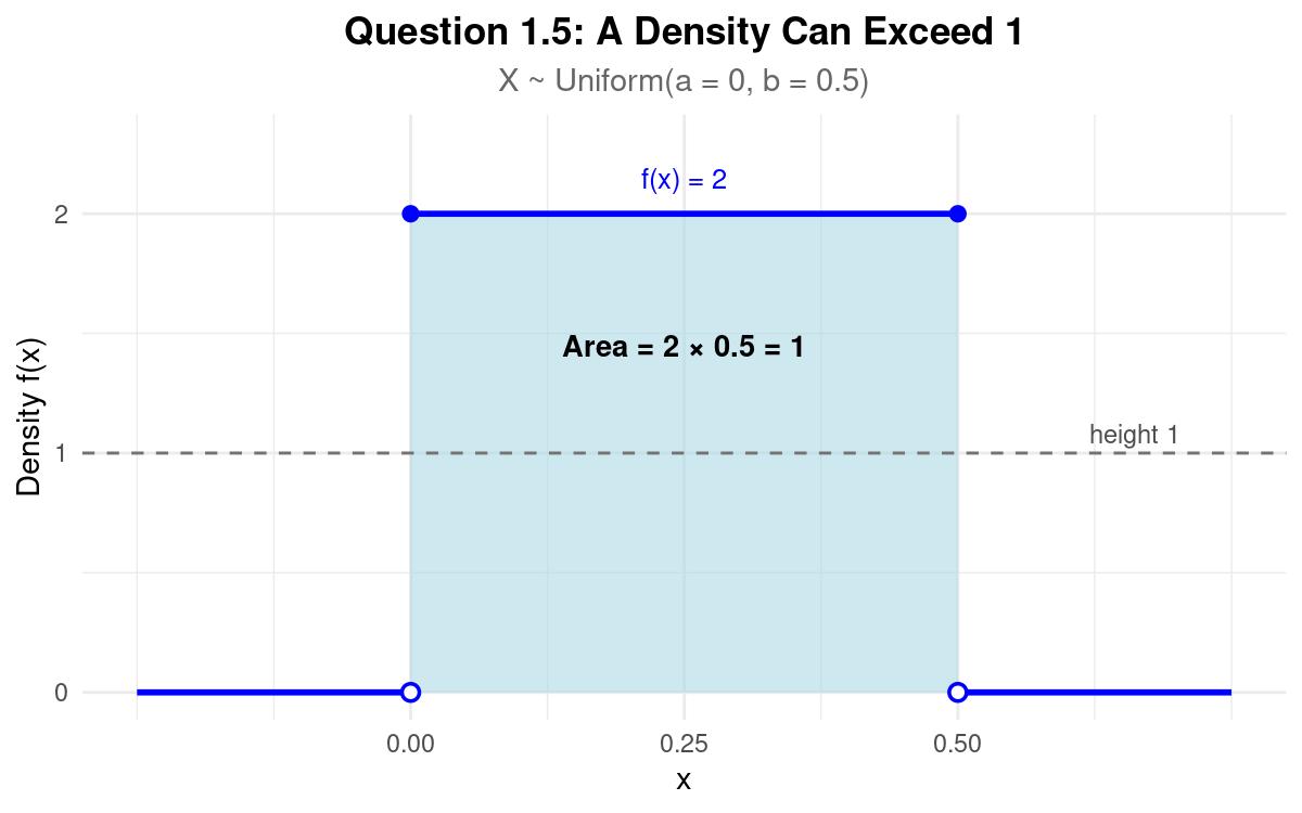
Describe this figure in detail

The horizontal axis shows x from about −0.25 to 0.75, and the vertical axis shows density from 0 to about 2.3. The density is 0 to the left of x = 0, jumps to height 2 at x = 0, stays at height 2 until x = 0.5, and drops back to 0 to the right of x = 0.5. Filled dots at height 2 and open dots at height 0 mark both endpoints. The rectangle under the segment, from x = 0 to x = 0.5 and from height 0 to height 2, is shaded and labeled “Area = 2 × 0.5 = 1.” A dashed horizontal line at height 1, labeled “height 1,” crosses the shaded rectangle halfway up.

Question 1.6 (2 pts)

Suppose \(X \sim N(\mu, \sigma^2)\).

True or False: The probability that \(X\) falls within \(1.28\) standard deviations of the mean, \(P(\mu - 1.28\sigma \leq X \leq \mu + 1.28\sigma)\), is \(0.80\).

Solution

Answer: TRUE

Standardize with \(Z = (X - \mu)/\sigma\) and use the standard normal table:

\[\begin{split}P(\mu - 1.28\sigma \leq X \leq \mu + 1.28\sigma) &= P(-1.28 \leq Z \leq 1.28) \\ &= \Phi(1.28) - \Phi(-1.28) \\ &= 0.8997 - 0.1003 = 0.7994 \approx 0.80.\end{split}\]

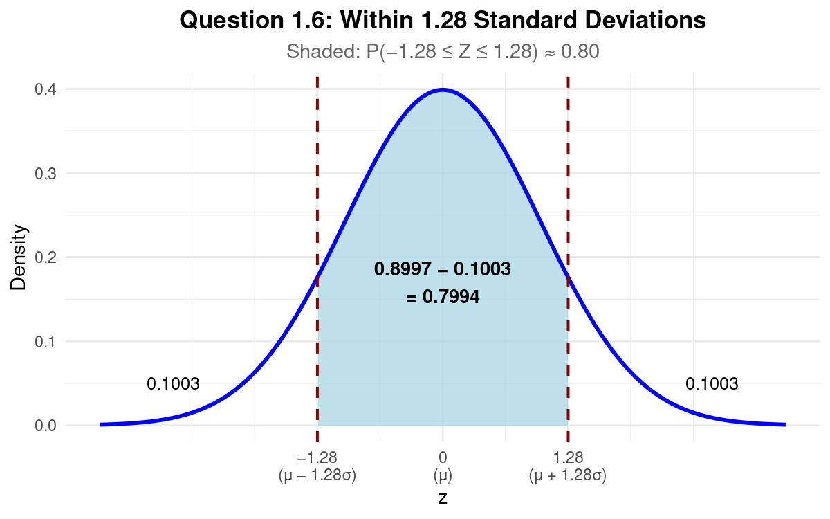
Describe this figure in detail

A bell-shaped standard normal curve is drawn over z values from −3.5 to 3.5 and peaks at 0.4 above z = 0. Dashed vertical lines stand at z = −1.28 and z = 1.28; the axis also labels them μ − 1.28σ and μ + 1.28σ, and labels z = 0 as μ. The region under the curve between the dashed lines is shaded and labeled “0.8997 − 0.1003 = 0.7994.” The two unshaded tails, to the left of −1.28 and to the right of 1.28, are each labeled 0.1003.

---

Problem 2 — Multiple Choice (15 points, 3 points each)

Question 2.1 (3 pts)

A survey of 150 recent Purdue engineering graduates revealed that their starting annual salaries had a sample mean of $86,500 and a sample median of $78,000. Based on these summary statistics, which of the following statements is most likely true regarding the distribution of starting salaries?

1. The distribution is symmetric and mound-shaped because engineering salaries are standardized.

2. The distribution is right-skewed (positively skewed) because a relatively small number of exceptionally high salaries pull the sample mean above the sample median.

3. The distribution is left-skewed (negatively skewed) because the majority of graduates earn less than the mean.

4. The sample standard deviation must be equal to zero.

5. The interquartile range (IQR) is guaranteed to be larger than the full range of the data.

Solution

Answer: (B)

• (A) FALSE. In a symmetric distribution the sample mean and sample median are close; here the sample mean is $8,500 above the sample median.

• (B) TRUE. The sample mean is sensitive to extreme values and the sample median is not. A few very high salaries pull the sample mean above the sample median, which is the pattern of a right-skewed distribution.

• (C) FALSE. In a left-skewed distribution, low values pull the sample mean below the sample median. Here the sample mean is above the sample median.

• (D) FALSE. A standard deviation of zero means every salary is the same, so the sample mean and sample median would be equal.

• (E) FALSE. The IQR can never exceed the range, because \(Q_1 \geq \min\) and \(Q_3 \leq \max\).

Question 2.2 (3 pts)

During peak lunch hours at the Purdue Memorial Union, mobile food orders arrive according to a Poisson process at an average rate of \(0.4\) orders per minute. What is the probability that exactly \(2\) orders arrive in a randomly selected \(5\)-minute interval?

1. 0.0544

2. 0.1465

3. 0.2707

4. 0.4000

5. 0.6767

Solution

Answer: (C)

A 5-minute interval has mean \(\lambda = 0.4 \times 5 = 2\) orders, so the number of orders \(X\) in the interval satisfies \(X \sim \text{Poisson}(\lambda = 2)\):

\[P(X = 2) = \frac{e^{-2}\,2^2}{2!} = 2e^{-2} = 0.2707.\]

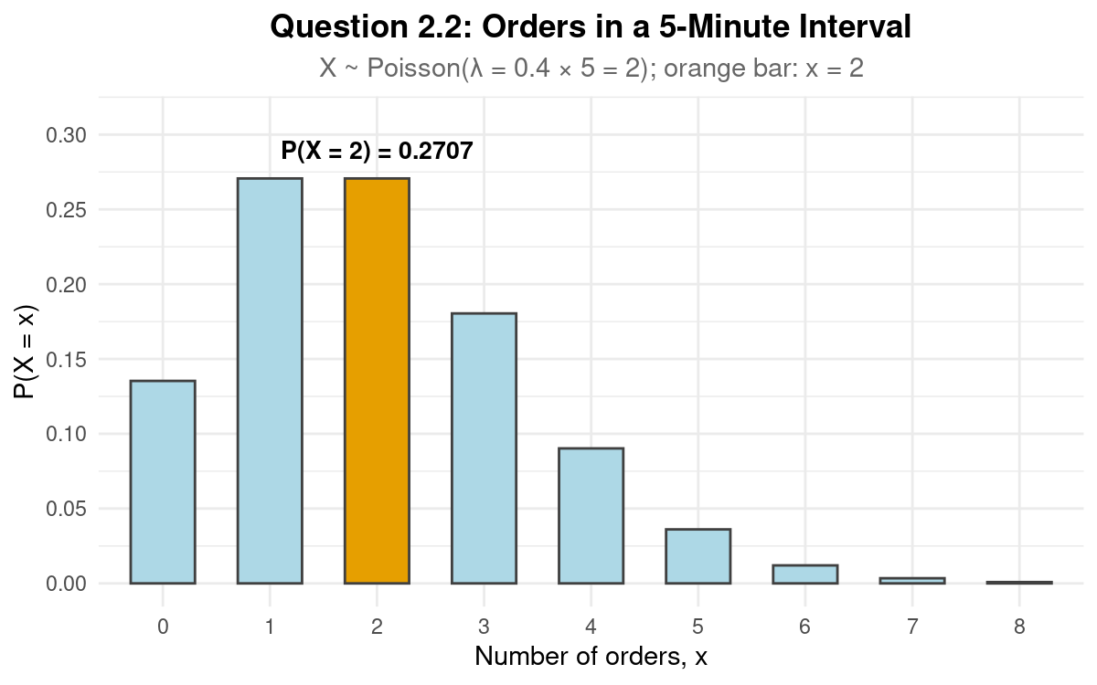
Describe this figure in detail

Bars stand at x = 0, 1, 2, …, 8 on the horizontal axis, with heights P(X = x) on the vertical axis from 0 to 0.30. The bars at x = 1 and x = 2 are the tallest and have the same height, 0.2707. The bar at x = 2 is orange and labeled “P(X = 2) = 0.2707”; all other bars are light blue. The bar at x = 0 is about 0.14. After x = 2 the heights fall: about 0.18 at x = 3, 0.09 at x = 4, and 0.04 at x = 5, and the bars at x = 7 and x = 8 are almost flat on the axis.

Question 2.3 (3 pts)

Let \(X\) be a discrete random variable representing the number of defective components found in an electronic assembly pack, with probability mass function:

\[P(X = 0) = 0.60, \quad P(X = 1) = 0.30, \quad P(X = 2) = 0.10\]

The repair cost (in dollars) for a pack is modeled by the function \(C(X) = 50 + 20X^2\). What is the expected repair cost \(E[C(X)]\)?

1. $50.00

2. $57.00

3. $60.00

4. $64.00

5. $78.00

Solution

Answer: (D)

By linearity of expectation, \(E[C(X)] = 50 + 20\,E[X^2]\). By LOTUS,

\[E[X^2] = 0^2(0.60) + 1^2(0.30) + 2^2(0.10) = 0 + 0.30 + 0.40 = 0.70.\]

Therefore \(E[C(X)] = 50 + 20(0.70) = 64\), an expected repair cost of $64.00.

Question 2.4 (3 pts)

An inspector examines a small shipment of \(N = 25\) laptops. Unbeknownst to the inspector, the shipment contains exactly \(4\) defective units. The inspector randomly selects \(n = 5\) laptops without replacement and counts the number of defective units \(X\) among the \(5\) sampled. Which of the following explains why \(X\) does NOT strictly follow a Binomial distribution?

1. The draws are dependent because each selection changes which laptops remain in the shipment.

2. A draw cannot have binary outcomes because defect status is learned only after inspection.

3. The number of trials is not fixed because the defect count is unknown before inspection.

4. The expected defect count cannot be computed before the inspector checks the selected laptops.

5. The variance must exceed the sample size because the inspector samples without replacement.

Solution

Answer: (A)

• (A) TRUE. Each laptop drawn changes what remains. The second laptop is defective with probability \(3/24\) if the first was defective and \(4/24\) if it was not, so the draws are dependent and the Independent criterion of BInS fails.

• (B) FALSE. Each laptop is either defective or not, so every draw has two outcomes. When the status is learned does not matter.

• (C) FALSE. The number of draws is fixed in advance at \(n = 5\).

• (D) FALSE. An expected value is computed from the distribution of \(X\) before any laptop is inspected, and it is not one of the BInS criteria.

• (E) FALSE. Nothing requires the variance of \(X\) to exceed the sample size, and the variance is not one of the BInS criteria.

Question 2.5 (3 pts)

The delivery time \(T\) (in minutes) for autonomous delivery robots on the Purdue campus follows an Exponential distribution with rate \(\lambda = 0.10\) per minute. The dining service promises a delivery fee refund if an order takes longer than \(c\) minutes. If they wish to issue refunds for only the top \(2.5\%\) slowest deliveries, what should the threshold \(c\) be?

1. 27.73 minutes

2. 29.96 minutes

3. 36.89 minutes

4. 39.12 minutes

5. 46.05 minutes

Solution

Answer: (C)

For \(T \sim \text{Exp}(\lambda = 0.10)\), \(P(T > t) = e^{-0.10t}\) for \(t \geq 0\). The threshold \(c\) satisfies \(P(T > c) = 0.025\):

\[e^{-0.10c} = 0.025 \quad\Rightarrow\quad c = \frac{-\ln(0.025)}{0.10} = \frac{3.6889}{0.10} = 36.89 \text{ minutes}.\]

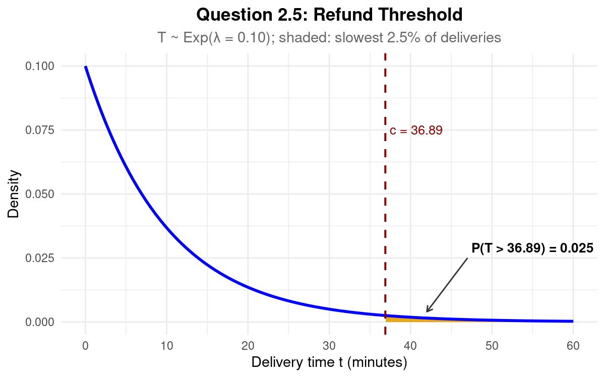
Describe this figure in detail

The horizontal axis shows delivery time t from 0 to 60 minutes, and the vertical axis shows density from 0 to 0.10. The curve starts at 0.10 when t = 0 and decreases steadily, lying close to the axis by t = 40. A dashed vertical line at t = 36.89 is labeled “c = 36.89.” The area under the curve to the right of that line is shaded orange; because the curve is so low there, the shaded region is a thin sliver along the axis. An arrow points to it from the label “P(T > 36.89) = 0.025.”

---

Problem 3 (26 points) — HPC Simulation Runtime

Problem 3 Setup

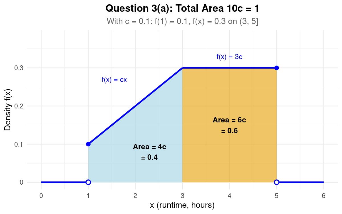
A High-Performance Computing (HPC) cluster at Purdue processes large-scale scientific simulations. Every submitted task runs a mandatory one-hour CPU calibration stage before its simulation can finish or reach a checkpoint. Let \(X\) denote the total active CPU runtime (in hours), including that calibration stage, of a randomly submitted simulation task before completion or checkpointing. Thus, \(X\) cannot be less than one hour. The probability density function (PDF) of \(X\) is modeled by the following piecewise function:

\[\begin{split}f(x) = \begin{cases} cx, & 1 \leq x \leq 3 \\ 3c, & 3 < x \leq 5 \\ 0, & \text{otherwise} \end{cases}\end{split}\]

Question 3a (8 pts)

Determine the value of the constant \(c\) such that \(f(x)\) is a valid probability density function. Show all integration steps clearly.

Solution

The total area under \(f\) must be 1:

\[1 = \int_1^3 cx\,dx + \int_3^5 3c\,dx = c\left[\frac{x^2}{2}\right]_1^3 + 3c\,\big[x\big]_3^5 = c\left(\frac{9}{2} - \frac{1}{2}\right) + 3c(5 - 3) = 4c + 6c = 10c.\]

Thus \(c = \dfrac{1}{10} = 0.1000\).

Describe this figure in detail

The horizontal axis shows runtime x from 0 to 6 hours, and the vertical axis shows density from 0 to about 0.38. The density is 0 for x below 1. At x = 1 it jumps to 0.1 (a filled dot at 0.1 and an open dot at 0), then rises in a straight line, labeled f(x) = cx, to 0.3 at x = 3. From x = 3 to x = 5 it stays flat at 0.3, labeled f(x) = 3c, then drops to 0 at x = 5 (a filled dot at 0.3 and an open dot at 0) and stays at 0. The region under the rising line, from x = 1 to x = 3, is shaded light blue and labeled “Area = 4c = 0.4.” The rectangle under the flat part, from x = 3 to x = 5, is shaded orange and labeled “Area = 6c = 0.6.”

Question 3b (6 pts)

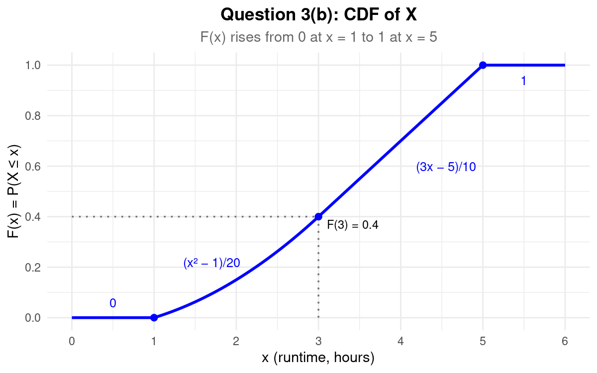
The intervals of the Cumulative Distribution Function \(F(x)\) are shown below. Find the expression for each labeled blank (i)–(iv) to complete \(F(x)\) for all real numbers \(x \in \mathbb{R}\).

\[\begin{split}F(x) = \begin{cases} \boxed{\text{(i)}} & x < 1 \\ \boxed{\text{(ii)}} & 1 \leq x \leq 3 \\ \boxed{\text{(iii)}} & 3 < x \leq 5 \\ \boxed{\text{(iv)}} & x > 5 \end{cases}\end{split}\]

Solution

No probability lies below 1, and all of it lies at or below 5, so the outer blanks are (i) \(0\) and (iv) \(1\). With \(c = \tfrac{1}{10}\), the two inner cases are:

\[\text{(ii)}\quad F(x) = \int_1^x \frac{t}{10}\,dt = \frac{x^2 - 1}{20},\]

\[\text{(iii)}\quad F(x) = F(3) + \int_3^x \frac{3}{10}\,dt = \frac{2}{5} + \frac{3(x - 3)}{10} = \frac{3x - 5}{10}.\]

The complete CDF is

\[\begin{split}F(x) = \begin{cases} 0 & x < 1 \\[4pt] \dfrac{x^2 - 1}{20} & 1 \leq x \leq 3 \\[8pt] \dfrac{3x - 5}{10} & 3 < x \leq 5 \\[8pt] 1 & x > 5 \end{cases}\end{split}\]

Describe this figure in detail

The horizontal axis shows x from 0 to 6, and the vertical axis shows F(x) = P(X ≤ x) from 0 to 1. F(x) is flat at 0 from x = 0 to x = 1. From x = 1 to x = 3 it bends upward along the curve labeled (x² − 1)/20 and reaches 0.4 at x = 3; dotted guide lines connect the point (3, 0.4) to both axes, and the point is labeled “F(3) = 0.4.” From x = 3 to x = 5 it rises in a straight line labeled (3x − 5)/10 and reaches 1 at x = 5, then stays flat at 1. The graph has no jumps.

Question 3c (4 pts)

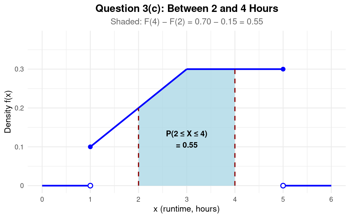
What is the probability that a randomly chosen simulation task takes between \(2\) and \(4\) hours to finish?

Solution

Using the two inner cases of \(F(x)\), \(F(4) = \tfrac{7}{10}\) and \(F(2) = \tfrac{3}{20}\). Hence,

\[P(2 \leq X \leq 4) = F(4) - F(2) = \frac{7}{10} - \frac{3}{20} = \frac{11}{20} = 0.5500.\]

Describe this figure in detail

The density from Question 3(a) is drawn again: 0 below x = 1, rising from 0.1 at x = 1 to 0.3 at x = 3, flat at 0.3 until x = 5, then 0. Dashed vertical lines stand at x = 2, where the density is 0.2, and at x = 4, where it is 0.3. The region under the density between the two dashed lines is shaded and labeled “P(2 ≤ X ≤ 4) = 0.55.” The regions from x = 1 to x = 2 and from x = 4 to x = 5 are unshaded.

Question 3d (4 pts)

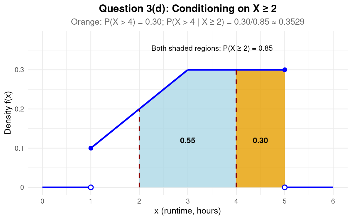
Given that a simulation task has already run for at least \(2\) hours, what is the conditional probability that it takes more than \(4\) hours to finish?

Solution

Since \(\{X > 4\} \subseteq \{X \geq 2\}\), the intersection of the two events is \(\{X > 4\}\):

\[P(X > 4 \mid X \geq 2) = \frac{P(X > 4)}{P(X \geq 2)} = \frac{1 - F(4)}{1 - F(2)} = \frac{0.3000}{0.8500} = \frac{6}{17} \approx 0.3529.\]

Describe this figure in detail

The same density is drawn, with dashed vertical lines at x = 2 and x = 4. The region under the density from x = 2 to x = 4 is shaded light blue and labeled 0.55. The region from x = 4 to x = 5 is shaded orange and labeled 0.30. Text above the density reads “Both shaded regions: P(X ≥ 2) = 0.85.” The region from x = 1 to x = 2 is unshaded. The subtitle gives \(P(X > 4 \mid X \geq 2) = 0.30/0.85 \approx 0.3529\), the orange area as a fraction of all the shaded area.

Question 3e (4 pts)

Find the median execution duration \(\tilde{\mu}\) (in hours) of a simulation task.

Solution

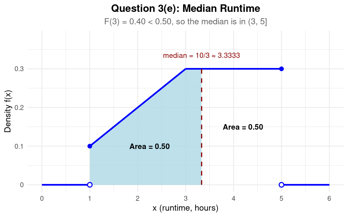
Since \(F(3) = 0.4000 < 0.50\), the median lies in \(3 < x \leq 5\). Solve

\[F(\tilde{\mu}) = \frac{3\tilde{\mu} - 5}{10} = 0.50 \quad\Rightarrow\quad \tilde{\mu} = \frac{10}{3} \approx 3.3333 \text{ hours}.\]

Describe this figure in detail

The same density is drawn. A dashed vertical line at x = 10/3 ≈ 3.3333, just to the right of x = 3 on the flat part of the density, is labeled “median = 10/3 ≈ 3.3333.” The region under the density from x = 1 to the dashed line is shaded and labeled “Area = 0.50.” The region from the dashed line to x = 5 is unshaded and is also labeled “Area = 0.50.”

---

Problem 4 (26 points) — Autonomous Shuttle Alerts

Problem 4 Setup

Purdue’s autonomous electric shuttle fleet navigates three campus routes: Route A (Engineering Quad), Route B (Stadium Drive), and Route C (Discovery Park).

Shuttles are assigned randomly to routes based on campus demand:

• Route A: assigned \(50\%\) of the time, \(P(A) = 0.50\)

• Route B: assigned \(30\%\) of the time, \(P(B) = 0.30\)

• Route C: assigned \(20\%\) of the time, \(P(C) = 0.20\)

During operation, high pedestrian density or sun glare may trigger a safety sensor alert (\(S\)). Telemetry data shows:

• On Route A: \(P(S \mid A) = 0.08\)

• On Route B: \(P(S \mid B) = 0.15\)

• On Route C: \(P(S \mid C) = 0.25\)

Question 4a (4 pts)

Calculate the joint probabilities for the three alert scenarios: \(P(A \cap S)\), \(P(B \cap S)\), and \(P(C \cap S)\).

Solution

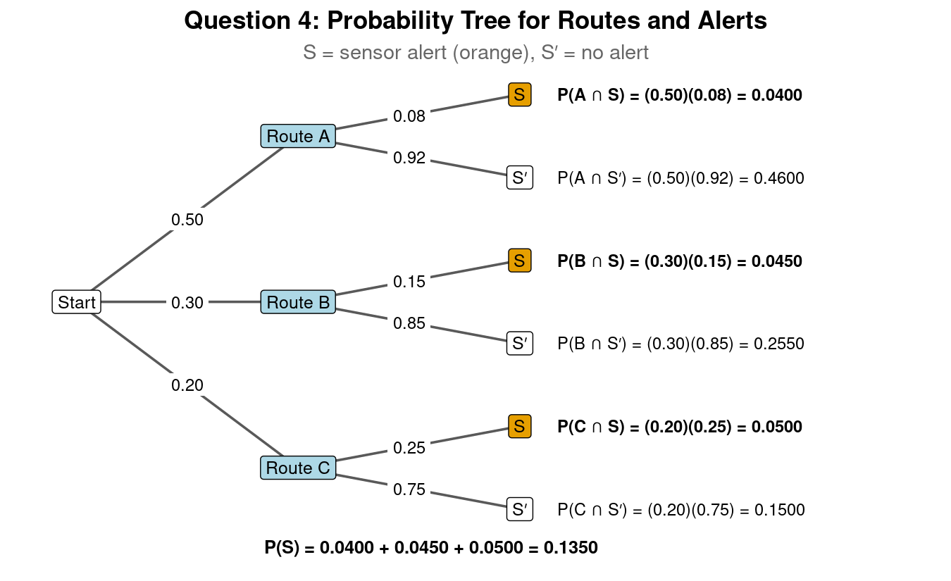
Apply \(P(R \cap S) = P(R)\,P(S \mid R)\) for each route \(R\):

\[\begin{split}P(A \cap S) &= (0.50)(0.08) = 0.0400 \\ P(B \cap S) &= (0.30)(0.15) = 0.0450 \\ P(C \cap S) &= (0.20)(0.25) = 0.0500\end{split}\]

Describe this figure in detail

The tree reads from left to right. From the node “Start,” three branches lead to “Route A” (labeled 0.50), “Route B” (0.30), and “Route C” (0.20). Each route node splits into two branches: an upper branch to S, a sensor alert, and a lower branch to S′, no alert. The branch probabilities are 0.08 and 0.92 for Route A, 0.15 and 0.85 for Route B, and 0.25 and 0.75 for Route C. At the end of each branch is its joint probability: P(A ∩ S) = (0.50)(0.08) = 0.0400, P(A ∩ S′) = (0.50)(0.92) = 0.4600, P(B ∩ S) = (0.30)(0.15) = 0.0450, P(B ∩ S′) = (0.30)(0.85) = 0.2550, P(C ∩ S) = (0.20)(0.25) = 0.0500, and P(C ∩ S′) = (0.20)(0.75) = 0.1500. The three S nodes are orange, and their joint probabilities are in bold. The line under the tree reads “P(S) = 0.0400 + 0.0450 + 0.0500 = 0.1350.”

Question 4b (6 pts)

Calculate the overall probability \(P(S)\) that a randomly selected shuttle trip experiences a sensor alert.

Solution

The three routes partition the sample space, so by the Law of Partitions,

\[P(S) = P(A \cap S) + P(B \cap S) + P(C \cap S) = 0.0400 + 0.0450 + 0.0500 = 0.1350.\]

Question 4c (8 pts)

Suppose a shuttle trip is known to have experienced a sensor alert (\(S\)). Compute the probability that this shuttle was traveling on Route A.

Solution

By Bayes’ Theorem,

\[P(A \mid S) = \frac{P(A \cap S)}{P(S)} = \frac{0.0400}{0.1350} = \frac{8}{27} \approx 0.2963.\]

Question 4d (5 pts)

Are the event \(\{\text{Shuttle is on Route A}\}\) and the event \(\{\text{Sensor alert occurs}\}\) independent? State YES or NO and provide clear mathematical justification.

Solution

NO. Since \(P(S \mid A) = 0.0800 \neq P(S) = 0.1350\), the two events are dependent. Equivalently, \(P(A \cap S) = 0.0400\), while \(P(A)\,P(S) = (0.50)(0.1350) = 0.0675\).

Question 4e (3 pts)

Suppose \(4\) independent shuttle trips on Route C are monitored. What is the probability that at least one of these \(4\) trips experiences a sensor alert?

Solution

Let \(Y\) be the number of the 4 trips with an alert. Each trip has an alert or not, the trips are independent, \(n = 4\) is fixed, and each trip has the same alert probability \(P(S \mid C) = 0.25\), so \(Y \sim \text{Binomial}(n = 4, p = 0.25)\). Use the complement:

\[P(Y \geq 1) = 1 - P(Y = 0) = 1 - (0.75)^4 = 1 - 0.3164 = 0.6836.\]

---

Problem 5 (26 points) — Silicon Wafer Thickness

Problem 5 Setup

High-precision silicon wafer substrates manufactured at the Birck Nanotechnology Center have a thickness \(X\) (in micrometers) that follows a Normal distribution with unknown mean \(\mu\) and unknown standard deviation \(\sigma\).

Quality assurance testing on a large production run establishes the following two specifications:

1. Exactly \(10\%\) of the manufactured wafers have a thickness strictly less than \(47.812\) micrometers: \(P(X < 47.812) = 0.10\).

2. Exactly \(5\%\) of the manufactured wafers have a thickness strictly greater than \(53.944\) micrometers: \(P(X > 53.944) = 0.05\).

Use a standard normal table with \(z\) values rounded to two decimal places. If two table entries are equally close to a target cumulative area, use the smaller \(z\) value.

Question 5a (8 pts)

Calculate the population mean \(\mu\) and standard deviation \(\sigma\).

Solution

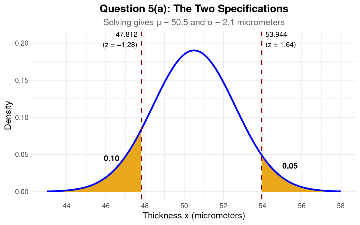
From the standard normal table, \(\Phi(-1.28) = 0.1003\) is the entry closest to 0.10, so \(z = -1.28\). Specification 2 gives a cumulative area of \(P(X \leq 53.944) = 0.95\); \(\Phi(1.64) = 0.9495\) and \(\Phi(1.65) = 0.9505\) are equally close, and the stated tie rule selects \(z = 1.64\). Thus,

\[47.812 = \mu - 1.28\sigma, \qquad 53.944 = \mu + 1.64\sigma.\]

Subtracting the first equation from the second gives \(6.132 = 2.92\sigma\), so

\[\sigma = \frac{53.944 - 47.812}{1.64 + 1.28} = \frac{6.132}{2.92} = 2.1 \text{ micrometers},\]

\[\mu = 47.812 + 1.28(2.1) = 50.5 \text{ micrometers}.\]

Describe this figure in detail

The horizontal axis shows thickness from 43 to 58 micrometers. A bell-shaped normal curve peaks above 50.5. A dashed vertical line at 47.812 is labeled z = −1.28, and the area under the curve to its left is shaded orange and labeled 0.10. A dashed vertical line at 53.944 is labeled z = 1.64, and the area to its right is shaded orange and labeled 0.05. The region between the two lines is unshaded.

Fallback values for 5(b)–5(d)

If you cannot determine \(\mu\) and \(\sigma\) in 5(a), you may use \(\mu = 50\) micrometers and \(\sigma = 2.0\) micrometers for parts 5(b)–5(d). These are not the correct answers to 5(a); they are provided only so you can continue with the rest of the problem. If you use them, say so clearly in your work. You will not receive credit for 5(a) by using these values.

Question 5b (6 pts)

Find the probability that a randomly chosen wafer has a thickness between \(47\) micrometers and \(53\) micrometers.

Solution

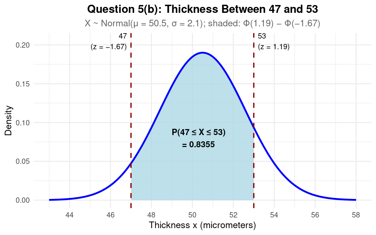
With \(\mu = 50.5\) and \(\sigma = 2.1\), the endpoints standardize to

\[z = \frac{47 - 50.5}{2.1} = -1.6667 \approx -1.67, \qquad z = \frac{53 - 50.5}{2.1} = 1.1905 \approx 1.19.\]

The table gives \(\Phi(-1.67) = 0.0475\) and \(\Phi(1.19) = 0.8830\), so

\[P(47 \leq X \leq 53) = \Phi(1.19) - \Phi(-1.67) = 0.8830 - 0.0475 = 0.8355.\]

With the fallback values, the endpoints standardize to \(z = -1.50\) and \(z = 1.50\), and \(P(47 \leq X \leq 53) = 0.9332 - 0.0668 = 0.8664\).

Describe this figure in detail

The same normal curve, peaking above 50.5, is drawn over 43 to 58 micrometers. Dashed vertical lines at 47 (labeled z = −1.67) and 53 (labeled z = 1.19) mark the interval. The area under the curve between them is shaded and labeled “P(47 ≤ X ≤ 53) = 0.8355.” The interval is not centered on the peak: 47 is 3.5 micrometers below 50.5, and 53 is 2.5 micrometers above it.

Question 5c (6 pts)

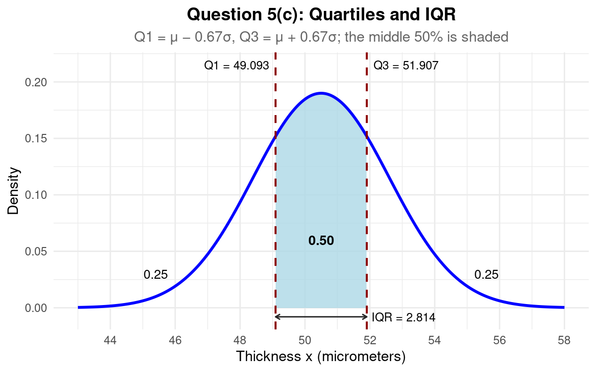
Determine the first quartile \(Q_1\), the third quartile \(Q_3\), and the population Interquartile Range (IQR) for wafer thickness.

Solution

The standard normal table gives \(\Phi(-0.67) = 0.2514\) and \(\Phi(0.67) = 0.7486\), the entries closest to 0.25 and 0.75, so use quartile \(z\) values \(\pm 0.67\):

\[\begin{split}Q_1 &\approx \mu - 0.67\sigma = 50.5 - 0.67(2.1) = 49.093 \text{ micrometers} \\ Q_3 &\approx \mu + 0.67\sigma = 50.5 + 0.67(2.1) = 51.907 \text{ micrometers} \\ \text{IQR} &= Q_3 - Q_1 = 2.814 \text{ micrometers}\end{split}\]

With the fallback values, \(Q_1 \approx 48.66\) micrometers, \(Q_3 \approx 51.34\) micrometers, and \(\text{IQR} \approx 2.68\) micrometers.

Describe this figure in detail

The same normal curve is drawn. Dashed vertical lines stand at Q1 = 49.093 and Q3 = 51.907, the same distance on either side of the peak at 50.5. The area under the curve between them is shaded and labeled 0.50. The two unshaded tails are each labeled 0.25. A double-headed arrow just below the axis runs from Q1 to Q3 and is labeled IQR = 2.814.

Question 5d (6 pts)

Calculate the population lower and upper inner fences. Using these fences as a quality-control rule, would a manufactured wafer with a thickness of \(44.20\) micrometers be flagged as a potential outlier requiring further inspection? Explain in a complete sentence.

Solution

\[\begin{split}\text{Lower inner fence} &= Q_1 - 1.5\,\text{IQR} = 49.093 - 1.5(2.814) = 44.872 \text{ micrometers} \\ \text{Upper inner fence} &= Q_3 + 1.5\,\text{IQR} = 51.907 + 1.5(2.814) = 56.128 \text{ micrometers}\end{split}\]

Because \(44.20\) micrometers is below the lower inner fence of \(44.872\) micrometers, the wafer would be flagged as a potential outlier.

With the fallback values, the fences are \(44.64\) and \(55.36\) micrometers. Because \(44.20 < 44.64\), the wafer would again be flagged as a potential outlier.

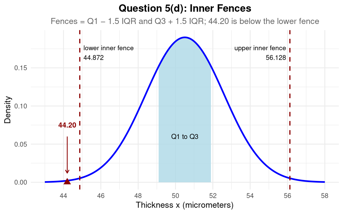
Describe this figure in detail

The same normal curve is drawn, with the region from Q1 to Q3 shaded and labeled “Q1 to Q3.” Dashed vertical lines at 44.872 and 56.128 are labeled “lower inner fence” and “upper inner fence.” Both fences lie far out in the tails, where the curve is close to the axis. A red triangle on the axis at 44.20, with an arrow pointing down to it from the label 44.20, sits to the left of the lower fence, outside the interval between the fences.