STAT 350 — Exam 1 — Spring 2026 (V1)

Exam Information

Course: STAT 350 — Introduction to Statistics

Semester: Spring 2026

Version: V1

Total Points: 105

Time Allowed: 60 minutes

Problem	Total Possible	Topic
Problem 1 (True/False, 2 pts each)	12	Continuous RVs, Binomial, Normal
Problem 2 (Multiple Choice, 3 pts each)	15	Discrete/Continuous RVs, Normal
Problem 3	15	Descriptive Statistics / Boxplots
Problem 4	26	Binomial Distribution, LOTUS
Problem 5	17	Conditional Probability / Independence
Problem 6	20	PDFs and CDFs
Total	105

---

Problem 1 — True/False (12 points, 2 points each)

Question 1.1 (2 pts)

Let \(X\) denote a continuous random variable with a PDF \(f_X(x)\). For any interval such that \([a, b] \subset \text{Support}(X)\), such that \(a < b\),

True or False: \(P(a < X < b)\) must be less than or equal to \(P(X < b)\).

Solution

Answer: TRUE

Since \(a < b\), the event \(\{a < X < b\}\) is a subset of the event \(\{X < b\}\). Specifically,

\[P(X < b) = P(X < a) + P(a \leq X < b) \geq P(a < X < b)\]

because \(P(X < a) \geq 0\). For any \(A \subseteq B\), we always have \(P(A) \leq P(B)\), so \(P(a < X < b) \leq P(X < b)\).

Question 1.2 (2 pts)

Suppose \(X\) is a Binomial random variable with parameters \(n\) and \(p\).

True or False: Holding the number of trials \(n\) constant, the shape of the distribution shifts from positively skewed to negatively skewed as \(p\) changes from 0.9 to 0.1.

Solution

Answer: FALSE

The direction of skew is reversed. When \(p\) is close to 1 (e.g., \(p = 0.9\)), most outcomes are large (near \(n\)), so the distribution is negatively skewed (long left tail). When \(p\) is close to 0 (e.g., \(p = 0.1\)), most outcomes cluster near 0, so the distribution is positively skewed (long right tail). Therefore, as \(p\) changes from 0.9 to 0.1, the distribution shifts from negatively to positively skewed — the opposite of what the statement claims.

Question 1.3 (2 pts)

Regarding the properties of a Binomial random variable \(X \sim \text{Binomial}(n, p)\).

True or False: The variance of \(X\) cannot exceed the number of independent trials \(n\).

Solution

Answer: TRUE

The variance of a Binomial random variable is \(\text{Var}(X) = np(1-p)\). Since \(0 < p < 1\), we have \(p(1-p) \leq \tfrac{1}{4}\), which gives

\[\text{Var}(X) = np(1-p) \leq n \cdot \tfrac{1}{4} \leq n.\]

Therefore, the variance cannot exceed \(n\).

Question 1.4 (2 pts)

Suppose \(V \sim \text{Binomial}(n, p)\) and \(W \sim \text{Poisson}(\lambda)\).

True or False: Then for any positive integer \(n\), the support of \(V\) is a subset of the support of \(W\).

Solution

Answer: TRUE

The support of \(V \sim \text{Binomial}(n, p)\) is \(\{0, 1, 2, \ldots, n\}\), a finite set. The support of \(W \sim \text{Poisson}(\lambda)\) is \(\{0, 1, 2, 3, \ldots\}\), the set of all non-negative integers. Since \(\{0, 1, \ldots, n\} \subseteq \{0, 1, 2, \ldots\}\) for any positive integer \(n\), the support of \(V\) is indeed a subset of the support of \(W\).

Question 1.5 (2 pts)

When converting a value \(x\) from a normal distribution into a \(z\)-score.

True or False: A negative \(z\)-score indicates that the original \(x\) is smaller than the population mean \(\mu\).

Solution

Answer: TRUE

The \(z\)-score is defined as \(z = \dfrac{x - \mu}{\sigma}\). Since \(\sigma > 0\), we have \(z < 0\) if and only if \(x - \mu < 0\), i.e., \(x < \mu\). A negative \(z\)-score therefore indicates the original value \(x\) lies below the population mean.

Question 1.6 (2 pts)

Suppose \(X\) and \(Y\) are Normally distributed random variables sharing the same mean \(\mu = 10\). It is also known that \(\text{Var}(X) < \text{Var}(Y)\).

True or False: Then it follows that \(P(X \leq 12)\) is larger than \(P(Y \leq 12)\).

Solution

Answer: TRUE

Since \(\text{Var}(X) < \text{Var}(Y)\), we have \(\sigma_X < \sigma_Y\). Converting 12 to a \(z\)-score for each:

\[z_X = \frac{12 - 10}{\sigma_X} = \frac{2}{\sigma_X}, \qquad z_Y = \frac{12 - 10}{\sigma_Y} = \frac{2}{\sigma_Y}.\]

Since \(\sigma_X < \sigma_Y\), we have \(z_X > z_Y > 0\). Because the standard normal CDF \(\Phi\) is increasing, \(\Phi(z_X) > \Phi(z_Y)\), which means \(P(X \leq 12) > P(Y \leq 12)\).

---

Problem 2 — Multiple Choice (15 points, 3 points each)

Question 2.1 (3 pts)

Let \(X\) and \(Y\) be discrete random variables that are not independent. Choose the statement about \(X\) and \(Y\) that always holds.

1. \(\text{Var}(X + Y) = \text{Var}(X) + \text{Var}(Y)\)

(B) For any \(x \in \text{Support}(X)\) and \(y \in \text{Support}(Y)\), \(P(X = x, Y = y) = P(X = x)P(Y = y)\).

3. \(E[XY] = E[X]E[Y]\)

4. \(E[X^3 + Y^{-2}] = E[X^3] + E[Y^{-2}]\)

5. \(\text{Cov}(X, Y) > 0\)

Solution

Answer: (D)

• (A) FALSE. In general, \(\text{Var}(X+Y) = \text{Var}(X) + \text{Var}(Y) + 2\,\text{Cov}(X,Y)\). Since \(X\) and \(Y\) are not independent, \(\text{Cov}(X,Y)\) need not be zero, so this equality does not always hold.

• (B) FALSE. This is the definition of independence, which is explicitly stated to be false here.

• (C) FALSE. \(E[XY] = E[X]E[Y]\) holds when \(\text{Cov}(X,Y) = 0\) (uncorrelated), but dependence does not guarantee this. In fact, \(E[XY] - E[X]E[Y] = \text{Cov}(X,Y)\), which may be nonzero.

• (D) TRUE. By the linearity of expectation, \(E[aX + bY] = aE[X] + bE[Y]\) holds for all random variables, regardless of dependence. Here, \(E[X^3 + Y^{-2}] = E[X^3] + E[Y^{-2}]\) always.

• (E) FALSE. Dependent random variables can have positive, negative, or zero covariance.

Question 2.2 (3 pts)

On days when STAT 350 homework is due, suppose Professor Reese receives extension requests according to a Poisson process at an average rate of 0.05 requests per 10 minutes. Compute the probability that he receives more than 1 extension request in a randomly selected 2-hour period.

1. 0.0012      (B) 0.0488      (C) 0.1219      (D) 0.4512      (E) 0.8781

Solution

Answer: (C)

A 2-hour period contains \(120 \div 10 = 12\) intervals of 10 minutes. The rate is 0.05 requests per 10-minute interval, so the expected number of requests in 2 hours is:

\[\lambda = 0.05 \times 12 = 0.6 \text{ requests}\]

Let \(X \sim \text{Poisson}(\lambda = 0.6)\). Then:

\[\begin{split}P(X > 1) &= 1 - P(X = 0) - P(X = 1) \\ &= 1 - e^{-0.6} - 0.6\,e^{-0.6} \\ &= 1 - e^{-0.6}(1 + 0.6) \\ &= 1 - (0.5488)(1.6) \\ &= 1 - 0.8781 \\ &= \boxed{0.1219}\end{split}\]

Question 2.3 (3 pts)

For some constant \(k\), define a PDF \(f_X(x) = k \cdot (x-5)^2\) for \(x \in [4, 6]\) and zero elsewhere. Which of the following statements correctly describes this distribution?

1. The distribution is bimodal.

2. The distribution is positively skewed.

3. The normalizing constant \(k\) can be negative.

4. The median is larger than the mean.

5. None of the above statements correctly describes the distribution.

Solution

Answer: (E)

First, find \(k\). Requiring \(\int_4^6 k(x-5)^2\,dx = 1\):

\[k \int_4^6 (x-5)^2\,dx = k\left[\frac{(x-5)^3}{3}\right]_4^6 = k\left(\frac{1}{3} + \frac{1}{3}\right) = \frac{2k}{3} = 1 \implies k = \frac{3}{2}.\]

Evaluate each option:

• (A) FALSE. The function \(f_X(x) = \tfrac{3}{2}(x-5)^2\) achieves its minimum value of 0 at \(x = 5\) and increases toward both endpoints \(x = 4\) and \(x = 6\). While the PDF is U-shaped, this does not constitute a bimodal distribution in the standard sense (bimodal requires two distinct interior local maxima).

• (B) FALSE. The PDF is symmetric about \(x = 5\) (since \((x-5)^2 = (5-x)^2\)), so the distribution is symmetric — neither positively nor negatively skewed.

• (C) FALSE. Since \((x-5)^2 \geq 0\) and \(f_X(x) \geq 0\) is required, \(k\) must be positive (\(k = \tfrac{3}{2} > 0\)).

• (D) FALSE. By symmetry of \(f_X(x)\) about \(x = 5\), the mean equals the median equals 5. The median is not larger than the mean.

• (E) TRUE. None of options (A)–(D) correctly describes this distribution.

Question 2.4 (3 pts)

The weights of packages shipped from a warehouse are Normally distributed with mean \(\mu = 50\) pounds (lbs) and standard deviation \(\sigma = 4\) lbs. A package is considered “light” if its weight is in the bottom 2.5% of the distribution. What is the cutoff weight to be considered a “light” package?

1. 38 lbs      (B) 40 lbs      (C) 42 lbs      (D) 44 lbs      (E) 46 lbs      (F) 48 lbs

Solution

Answer: (C)

We need the 2.5th percentile of \(\text{Normal}(\mu = 50, \sigma = 4)\). Let \(c\) be the cutoff weight. Then \(P(X \leq c) = 0.0250\).

From the \(z\)-table: \(\Phi(-1.96) = 0.0250\), so \(z = -1.96\).

Converting back to the original scale:

\[c = \mu + z\sigma = 50 + (-1.96)(4) = 50 - 7.84 = 42.16 \approx \boxed{42 \text{ lbs}}\]

Question 2.5 (3 pts)

Let \(T\) represent the “Triage Window” (in minutes) for resolving IT tickets at Purdue University. Suppose \(T\) follows a Normal distribution where it is known that \(P(T > 15) = 0.0668\) and \(P(T < 5) = 0.1587\). What is the mean \(\mu\) and standard deviation \(\sigma\) of this distribution?

1. \(\mu = 8,\ \sigma = 3.5\)      (B) \(\mu = 9,\ \sigma = 4\)      (C) \(\mu = 10,\ \sigma = 2\)      (D) \(\mu = 10,\ \sigma = 5\)

Solution

Answer: (B)

Setting up two equations. Convert each tail probability to a \(z\)-score using the \(z\)-table:

• \(P(T > 15) = 0.0668 \Rightarrow P(T \leq 15) = 0.9332\). From the table, \(\Phi(1.50) = 0.9332\), so \(z = 1.50\).

• \(P(T < 5) = 0.1587\). From the table, \(\Phi(-1.00) = 0.1587\), so \(z = -1.00\).

This gives the system:

\[\frac{15 - \mu}{\sigma} = 1.50 \quad \Rightarrow \quad 15 - \mu = 1.5\sigma \tag{1}\]

\[\frac{5 - \mu}{\sigma} = -1.00 \quad \Rightarrow \quad 5 - \mu = -\sigma \tag{2}\]

Solving. Subtract equation (2) from equation (1):

\[(15 - \mu) - (5 - \mu) = 1.5\sigma - (-\sigma) \implies 10 = 2.5\sigma \implies \sigma = 4.\]

Substituting back into (2): \(5 - \mu = -4 \Rightarrow \mu = 9\).

\[\boxed{\mu = 9, \quad \sigma = 4}\]

---

Problem 3 (15 points) — Screen Time Boxplot

Problem 3 Setup

A psychological research group studies the change in university students’ screen time and how this affects their studying patterns. As part of the study, they collected the screen time, in minutes, of 47 students. Below is a partial data table containing the sorted observations and a corresponding partial modified boxplot.

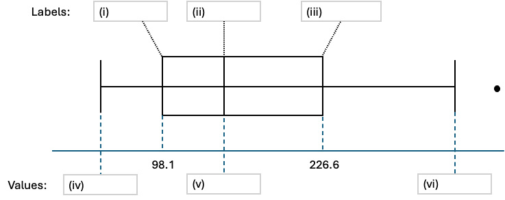
Question 3a (6 pts)

Fill in the blank spaces (i) – (vi) corresponding to the boxplot. For boxes (i), (ii), and (iii), provide the correct statistical terminology. For boxes (iv), (v), and (vi), provide the exact numerical value.

Solution

Terminology labels (top of boxplot):

• (i): First quartile \(Q_1\)

• (ii): Median \(Q_2\)

• (iii): Third quartile \(Q_3\)

Numerical values (bottom of boxplot):

• (iv): \(42.5\) (lower whisker / minimum — no observations fall below the lower fence)

• (v): \(145.3\) (the median, which is the 24th observation in a sorted sample of \(n = 47\))

• (vi): \(342.8\) (upper whisker — 487.2 is an explicit outlier plotted beyond the whisker)

Justification for (v): The median position for \(n = 47\) is \(\tfrac{47+1}{2} = 24\), so the median is the 24th sorted observation = 145.3.

Justification for (vi): The upper fence is \(Q_3 + 1.5 \times \text{IQR} = 226.6 + 1.5(128.5) = 226.6 + 192.75 = 419.35\). Since \(487.2 > 419.35\), the value 487.2 is plotted as an explicit outlier and the upper whisker extends to the largest non-outlier observation, 342.8.

Question 3b (3 pts)

Based on the distribution shown, where is the mean for this dataset most likely to exist?

1. Between the minimum and first quartile.

2. Between the first quartile and the median.

3. Between the median and third quartile.

4. Between the third quartile and maximum.

5. No single option is more likely than others.

Solution

Answer: (D)

The boxplot reveals strong right skew: the right whisker is considerably longer than the left whisker, and there is a high outlier at 487.2. In a right-skewed distribution, the mean is pulled toward the long right tail and typically exceeds the median. The extreme outlier at 487.2 (far above the upper whisker of 342.8) exerts substantial upward leverage on the mean, pulling it above \(Q_3 = 226.6\) and into the region between the third quartile and the maximum.

Question 3c (3 pts)

Compute the interquartile range (IQR). Explain its significance strictly in the context of the students’ screen time data.

Solution

\[\text{IQR} = Q_3 - Q_1 = 226.6 - 98.1 = \boxed{128.5 \text{ minutes}}\]

Interpretation: The IQR of 128.5 minutes means that the middle 50% of students’ screen times span a range of approximately 128.5 minutes. In other words, the student at the 75th percentile of screen time watches about 128.5 more minutes per day than the student at the 25th percentile.

Question 3d (3 pts)

Approximately how many data points are at least 98.1 and at most 226.6?

Solution

The interval \([98.1,\ 226.6] = [Q_1, Q_3]\) contains the middle 50% of the observations. Therefore:

\[0.50 \times 47 \approx \boxed{24} \text{ data points}\]

---

Problem 4 (26 points) — Defective Components

Problem 4 Setup

Due to recent severe mechanical failures on the assembly line, a production facility is experiencing an unusually high rate of errors. A quality inspector examines a small batch of \(n = 4\) electronic components from a massive production line. Each component independently has a probability \(p = 0.3\) of being defective. Let \(X\) denote the number of defective components in the batch.

Question 4a (4 pts)

Identify the distribution of \(X\), including its parameter(s). Write out the exact PMF formula for \(P(X = x)\) and state the support of \(X\).

Solution

\(X \sim \text{Binomial}(n = 4,\ p = 0.3)\)

Support: \(X \in \{0, 1, 2, 3, 4\}\)

PMF:

\[P(X = x) = \binom{4}{x} (0.3)^x (0.7)^{4-x}, \quad x \in \{0, 1, 2, 3, 4\}\]

The conditions for a Binomial model are satisfied: fixed number of trials (\(n = 4\)), each component is independently defective with the same probability \(p = 0.3\), and each trial results in success (defective) or failure (non-defective).

Question 4b (5 pts)

Compute the probability of observing at least two defective components in the batch.

Solution

\[\begin{split}P(X \geq 2) &= 1 - P(X = 0) - P(X = 1) \\[6pt] P(X = 0) &= (0.7)^4 = 0.2401 \\[4pt] P(X = 1) &= \binom{4}{1}(0.3)^1(0.7)^3 = 4(0.3)(0.343) = 0.4116 \\[8pt] P(X \geq 2) &= 1 - 0.2401 - 0.4116 = \boxed{0.3483}\end{split}\]

Question 4c (5 pts)

Determine the expected number of defective components, the expected number of non-defective components, and the variance.

Solution

Expected number of defective components:

\[E[X] = np = 4(0.3) = \boxed{1.2}\]

Expected number of non-defective components:

\[E[n - X] = n - E[X] = n(1 - p) = 4(0.7) = \boxed{2.8}\]

Variance (the variance of both \(X\) and \(n - X\) is the same):

\[\text{Var}(X) = np(1-p) = 4(0.3)(0.7) = \boxed{0.84}\]

Question 4d (12 pts)

Suppose the automated QA machine scans the batches. If a batch has many defects, the automated QA machine halts early and rejects it. The diagnostic time (in minutes) spent on a batch is modeled by the function \(D = \dfrac{60}{X + 1}\). Calculate the expected diagnostic time, \(E[D]\). (Hint: The LOTUS flower brings clarity.)

Solution

Using the Law of the Unconscious Statistician (LOTUS):

\[E[D] = E\!\left[\frac{60}{X+1}\right] = \sum_{x=0}^{4} \frac{60}{x+1} \cdot P(X = x)\]

Step 1 — Compute all PMF values:

\(x\)	\(P(X = x)\)	\(\dfrac{60}{x+1}\)	\(\dfrac{60}{x+1} \cdot P(X=x)\)
0	\((0.7)^4 = 0.2401\)	60	14.4060
1	\(4(0.3)(0.7)^3 = 0.4116\)	30	12.3480
2	\(6(0.3)^2(0.7)^2 = 0.2646\)	20	5.2920
3	\(4(0.3)^3(0.7) = 0.0756\)	15	1.1340
4	\((0.3)^4 = 0.0081\)	12	0.0972

Step 2 — Sum:

\[E[D] = 14.4060 + 12.3480 + 5.2920 + 1.1340 + 0.0972 = \boxed{33.2772 \text{ minutes}}\]

---

Problem 5 (17 points) — Meredith the Cat

Problem 5 Setup

Meredith 🐱 follows a daily routine in the following order: eat → drink → poop → cuddle → sleep. If Meredith successfully completes the first four steps, she falls asleep and is happy 😺. If any of the steps are broken, Meredith is guaranteed to get mad 😾.

Let \((M)\) be the event that Meredith gets mad 😾; otherwise she is happy 😺 (falls asleep). Let \(E\), \(D\), \(P\), and \(C\) be the events that the routine is broken at the eat, drink, poop, and cuddle step, respectively. From an observational study, Meredith’s owner, Heekyung, learned that \(P(M) = 0.2\). When Meredith gets mad, the cause of the broken routine is 50% eat, 25% drink, 10% poop, and 15% cuddle.

Known probabilities:

\[P(M) = 0.2, \quad P(H) = 0.8\]

\[P(E \mid M) = 0.50, \quad P(D \mid M) = 0.25, \quad P(P \mid M) = 0.10, \quad P(C \mid M) = 0.15\]

Question 5a (5 pts)

What is the probability that Meredith gets mad and the broken routine is “poop”?

Solution

Using the Multiplication Rule:

\[P(M \cap P) = P(P \mid M) \cdot P(M) = 0.10 \times 0.2 = \boxed{0.0200}\]

Question 5b (5 pts)

What is the probability that the broken routine is “eat” given that Meredith is happy?

Solution

Answer: \(P(E \mid H) = \boxed{0}\)

If Meredith is happy (i.e., she falls asleep), then by definition no step in her routine was broken. Therefore, the event \(E\) (eat routine is broken) and the event \(H\) (Meredith is happy) are mutually exclusive: \(E \cap H = \emptyset\). It follows that \(P(E \mid H) = 0\).

Question 5c (5 pts)

What is the probability that Meredith gets mad given that the “poop” routine is broken?

Solution

Answer: \(P(M \mid P) = \boxed{1}\)

The problem states: “If any of the steps are broken, Meredith is guaranteed to get mad.” Therefore, breaking the poop routine is a sufficient condition for getting mad. Since the poop step being broken (\(P\)) implies mad (\(M\)), we have \(P \subseteq M\) and thus \(P(M \mid P) = 1\).

Question 5d (2 pts)

Determine whether the events \(M\) and \(P\) are independent or not.

1. The two events are independent.

2. Two events are dependent.

Solution

Answer: (B) — Two events are dependent.

Two events are independent if and only if \(P(M \cap P) = P(M) \cdot P(P)\).

First compute \(P(P)\) using the Law of Total Probability:

\[P(P) = P(P \mid M)\,P(M) + P(P \mid H)\,P(H) = 0.10(0.2) + 0(0.8) = 0.02\]

Check independence:

\[P(M) \cdot P(P) = 0.2 \times 0.02 = 0.004\]

But from part (a): \(P(M \cap P) = 0.02 \neq 0.004\).

Since \(P(M \cap P) \neq P(M) \cdot P(P)\), the events \(M\) and \(P\) are dependent.

(Equivalently: :math:`P(M mid P) = 1 neq 0.2 = P(M)`)

---

Problem 6 (20 points) — GPU Thermal Stress Test

Problem 6 Setup

A data science lab is running a mandatory 10-hour thermal stress test on a new cluster of machine learning GPUs. Let \(T\) be the time (in hours) until a defective GPU fails during the test.

• Phase 1 (\(0 \leq t \leq 1\)): The thermal load ramps up linearly for the first hour.

• Phase 2 (\(1 < t \leq 10\)): The probability of failure decays smoothly according to an inverse-square law.

• The Cutoff: The stress test is automatically halted at exactly 10 hours.

The probability density function (PDF) for the failure time is modeled by:

\[\begin{split}f_T(t) = \begin{cases} \dfrac{5}{7} \cdot t & 0 \leq t \leq 1 \\[8pt] \dfrac{5}{7} \cdot \dfrac{1}{t^2} & 1 < t \leq 10 \\[8pt] 0 & \text{otherwise} \end{cases}\end{split}\]

Question 6a (10 pts)

The partially completed cumulative distribution function (CDF) is given below. Find the missing equation for the region between 1 and 10.

\[\begin{split}F_T(t) = \begin{cases} 0 & t < 0 \\[4pt] \dfrac{5}{14}\,t^2 & 0 \leq t < 1 \\[8pt] \text{[MISSING]} & 1 \leq t < 10 \\[4pt] 1 & t \geq 10 \end{cases}\end{split}\]

Solution

For \(1 \leq t < 10\), the CDF must accumulate probability from both regions. We carry forward the probability already accumulated through Phase 1, then add the integral over Phase 2 up to \(t\):

\[P(T \leq 1) = F_T(1) = \frac{5}{14}(1)^2 = \frac{5}{14}\]

\[F_T(t) = \underbrace{F_T(1)}_{\text{Phase 1}} + \int_1^t \frac{5}{7} \cdot \frac{1}{x^2}\,dx\]

Compute the integral explicitly:

\[\int_1^t \frac{5}{7} \cdot \frac{1}{x^2}\,dx = \frac{5}{7}\left[-\frac{1}{x}\right]_1^t = \frac{5}{7}\left(-\frac{1}{t} + 1\right) = \frac{5}{7} - \frac{5}{7t}\]

Combining:

\[F_T(t) = \frac{5}{14} + \frac{5}{7} - \frac{5}{7t} = \frac{5}{14} + \frac{10}{14} - \frac{5}{7t} = \boxed{\frac{15}{14} - \frac{5}{7t}}, \quad 1 \leq t < 10\]

Verification: At \(t = 10\): \(\dfrac{15}{14} - \dfrac{5}{70} = \dfrac{15}{14} - \dfrac{1}{14} = \dfrac{14}{14} = 1\) ✓

---

\[\begin{split}F_T(t) = \begin{cases} 0 & t < 0 \\[4pt] \dfrac{5}{14}\,t^2 & 0 \leq t < 1 \\[8pt] \dfrac{15}{14} - \dfrac{5}{7t} & 1 \leq t < 10 \\[4pt] 1 & t \geq 10 \end{cases}\end{split}\]

---

Question 6b (10 pts)

Calculate the median failure time for a defective GPU.

Solution

We need \(\tilde{t}\) such that \(F_T(\tilde{t}) = 0.5\).

Step 1 — Identify which region contains the median.

At the boundary \(t = 1\):

\[F_T(1) = \frac{5}{14} \approx 0.3571 < 0.5\]

Since we do not reach probability 0.5 within the first phase (\(0 \leq t \leq 1\)), the median must lie in the Phase 2 region (\(1 \leq t < 10\)).

Step 2 — Solve for the median using the Phase 2 CDF.

\[\frac{15}{14} - \frac{5}{7\tilde{t}} = \frac{1}{2}\]

\[\frac{5}{7\tilde{t}} = \frac{15}{14} - \frac{1}{2} = \frac{15}{14} - \frac{7}{14} = \frac{8}{14} = \frac{4}{7}\]

\[\tilde{t} = \frac{5}{7} \cdot \frac{7}{4} = \frac{5}{4} = \boxed{1.25 \text{ hours}}\]

Verification: \(F_T(1.25) = \dfrac{15}{14} - \dfrac{5}{7(1.25)} = \dfrac{15}{14} - \dfrac{5}{8.75} = \dfrac{15}{14} - \dfrac{4}{7} = \dfrac{15}{14} - \dfrac{8}{14} = \dfrac{7}{14} = 0.5\) ✓