STAT 350 — Exam 2 — Spring 2024

Exam Information

Course: STAT 350 — Introduction to Statistics

Semester: Spring 2024

Total Points: 105

Time Allowed: 60 minutes

Problem	Total Possible	Topic
Problem 1 (True/False, 2 pts each)	12	Sampling Distributions, Inference, Experimental Design
Problem 2 (Multiple Choice, 3 pts each)	9	Experimental Design, CLT, Two-Sample Inference
Problem 3	32	Paired t-test, Power Analysis
Problem 4	20	CLT, Sampling Distribution of \(\bar{X}\)
Problem 5	32	One-Sample t-test, Confidence Bound
Total	105

---

Problem 1 — True/False (12 points, 2 points each)

Question 1.1 (2 pts)

If a simple random sample is taken from a normally distributed population,

True or False: then the distribution of the sample means follows a normal distribution, regardless of the sample size.

Solution

Answer: TRUE

When the population is normally distributed, the sampling distribution of \(\bar{X}\) is exactly normal for any sample size \(n \geq 1\). This follows directly from the property that any linear combination of independent normal random variables is also normal. The Central Limit Theorem is not needed here — it is the CLT that handles the non-normal population case.

Question 1.2 (2 pts)

If a simple random sample of size 2 or greater is taken from a normally distributed population,

True or False: then the variance of the sample mean is always greater than the population variance.

Solution

Answer: FALSE

The variance of the sample mean is \(\text{Var}(\bar{X}) = \sigma^2/n\). For any \(n \geq 2\), we have \(\sigma^2/n \leq \sigma^2/2 < \sigma^2\). The variance of \(\bar{X}\) is therefore strictly less than the population variance \(\sigma^2\), not greater.

Question 1.3 (2 pts)

In a simulation run where differences arise from a normal distribution in a paired sample procedure, and 92% confidence intervals are constructed for the mean difference across 1000 independent sets of paired samples,

True or False: exactly 80 of these intervals will not contain the true mean difference.

Solution

Answer: FALSE

A 92% confidence interval procedure means that, in the long run, 92% of intervals will contain the true mean difference and 8% will not. For 1000 independent intervals, we expect \(0.08 \times 1000 = 80\) to miss — but this is a random quantity. The actual number follows a \(\text{Binomial}(1000, 0.08)\) distribution, so it will not be exactly 80 in every simulation run.

Question 1.4 (2 pts)

When the significance level (\(\alpha\)) of a statistical test is reduced while holding all other factors constant,

True or False: the power of the test increases.

Solution

Answer: FALSE

Reducing \(\alpha\) makes the rejection region smaller (the critical value moves further into the tail), so it becomes harder to reject \(H_0\). This increases the probability of a Type II error (\(\beta\)) and therefore decreases power \((= 1 - \beta)\). There is an inherent trade-off: lowering \(\alpha\) reduces Type I error at the cost of reduced power.

Question 1.5 (2 pts)

In a two-sample independent t-test using the Welch procedure to account for unequal variances between groups,

True or False: the test statistic is assumed to adhere to an exact t-distribution, provided the assumption of normality holds.

Solution

Answer: FALSE

The Welch procedure uses the Welch–Satterthwaite approximation to compute the effective degrees of freedom. This approximation means the test statistic only approximately follows a t-distribution — it is not exact, even under normality. This is in contrast to the pooled two-sample t-test (equal variances assumed), which does follow an exact t-distribution under normality.

Question 1.6 (2 pts)

In a completely randomized experimental design,

True or False: random assignment of experimental units to treatments helps to minimize potential biases by helping to distribute extraneous variables more evenly across treatment groups.

Solution

Answer: TRUE

Random assignment is a core principle of experimental design precisely because it tends to balance both known and unknown extraneous variables across treatment groups by chance, thereby reducing the possibility of systematic bias. This is what allows causal conclusions to be drawn from a well-designed randomized experiment.

---

Problem 2 — Multiple Choice (9 points, 3 points each)

Question 2.1 (3 pts)

In a randomized block design, when we block experimental units based on a specific characteristic, the primary objective is to:

(A) Increase the variability arising from extraneous variables by grouping similar experimental units into blocks, thereby enhancing the detection of treatment effects.

(B) Decrease the variability arising from extraneous variables by grouping similar experimental units into blocks, thereby enhancing the detection of treatment effects.

(C) To allocate treatments to experimental units across blocks in a manner that conceals the treatment identities from both the participants and researchers.

(D) Equalize the allocation of treatments to experimental units within each block to facilitate the administrative convenience of the experiment.

(E) Balance the number of experimental units across blocks to primarily focus on the uniformity of treatment application without direct concern for extraneous or confounding variables.

Solution

Answer: (B)

The purpose of blocking is to reduce unwanted variability by grouping experimental units that are similar on a potential confounding characteristic into the same block. Because units within a block are more homogeneous, differences between blocks are removed from the error, making it easier to detect treatment effects against a smaller background of noise. Option (A) has the direction of variability wrong. Options (C)–(E) describe blinding, convenience, or uniformity — none of which is the primary objective of blocking.

Question 2.2 (3 pts)

Suppose a simple random sample of size 400 is taken from a skewed population with a known population mean of 200 units and a population standard deviation of 50 units. Which of the following statements is TRUE regarding the standard deviation of the sample mean?

(A) The standard deviation of the sample mean is equal to the population standard deviation, which is 50 units.

(B) The standard deviation of the sample mean cannot be accurately determined from the given information due to the population’s skewed distribution.

(C) The standard deviation of the sample mean, indicative of the sampling distribution’s variability, amounts to 0.125 units.

(D) The standard deviation of the sample mean is as large as 2500 units, indicative of the sampling distribution’s total variability.

(E) The standard deviation of the sample mean, indicative of the sampling distribution’s variability, amounts to 2.5 units.

Solution

Answer: (E)

The standard deviation of the sample mean (the standard error) is:

\[\sigma_{\bar{X}} = \frac{\sigma}{\sqrt{n}} = \frac{50}{\sqrt{400}} = \frac{50}{20} = 2.5 \text{ units}\]

The shape of the population (skewed) is irrelevant for calculating the standard error — the formula \(\sigma/\sqrt{n}\) holds regardless of the population’s distribution, as long as \(\sigma\) is known. Option (B) is a common misconception.

Question 2.3 (3 pts)

When estimating the difference between two population means using confidence intervals, if a researcher incorrectly uses a pooled variance estimator under the false assumption of equal variances, despite the populations having unequal variances, how does this affect the margin of error for the confidence interval?

(A) The margin of error is unaffected, as the pooled estimator adjusts for variance differences.

(B) The margin of error decreases, reflecting an underestimated standard error due to the assumption violation.

(C) The margin of error increases, reflecting an overestimated standard error due to the assumption violation.

(D) The margin of error may inaccurately reflect the true variability, underestimating or overestimating it based on the sample sizes and actual variances.

(E) The margin of error becomes zero, indicating a failure of the pooled estimator to account for variance differences.

Solution

Answer: (D)

When the equal-variance assumption is violated, the pooled variance estimator blends the two sample variances using a weighted average. Depending on whether the larger variance group has a larger or smaller sample size, the pooled estimate may be either too large or too small relative to the true variability. Therefore, the margin of error may either over- or underestimate the true margin of error — the direction is not determined without knowing the specific sample sizes and the ratio of the true variances.

---

Problem 3 (32 points) — Marshmallow Study: Paired Design and Power

Problem 3 Setup

According to the famous Stanford marshmallow study, children’s ability to wait longer for rewards is positively correlated with their educational achievements. However, subsequent research has identified several factors, such as family background, home environment, and cultural differences, that might influence both a child’s waiting time for rewards and their educational achievements.

Question 3a (3 pts)

Which of the following statements is false?

(A) The positive correlation ensures causation because the marshmallow experiment is conducted before observing their educational achievements.

2. The positive correlation might be insignificant after considering lurking variables.

3. The underlying factors are lurking variables in the famous marshmallow study.

4. None of the above

Solution

Answer: (A)

Temporal precedence (the experiment occurring before the outcome) is a necessary condition for causation, but it is not sufficient. The marshmallow study is observational in nature with respect to educational outcomes — children were not randomly assigned to wait or not wait. The correlation between waiting time and educational achievement could be driven by lurking variables (family background, home environment, cultural factors) that influence both. Correlation never guarantees causation.

Options (B) and (C) are both true: the lurking variables could attenuate the correlation, and those factors (family background, home environment, cultural differences) are correctly identified as lurking variables.

Question 3b (3 pts)

A researcher is investigating the connection between the birth order of children and their ability to wait longer for rewards. The study will involve 15 randomly chosen households within the Greater Lafayette area, each with at least two children. For each household, the first and second child will be included in the experiment.

In the study, which of the following variables is NOT indirectly controlled by the paired design?

1. Parent’s occupation

2. Child’s birth order

3. Cultural background

4. Home environment

Solution

Answer: (B)

Pairing by household indirectly controls for variables that are shared within a household: parent’s occupation (A), cultural background (C), and home environment (D) are all held approximately constant for the two children in the same house. Birth order (B) is the explanatory variable of interest — it is the variable being studied, not a nuisance variable being controlled.

Question 3c (3 pts)

The researcher believes that the first child will wait longer for the rewards than the second child. Drawing on previous research, the standard deviation of the waiting time difference between the first and second children is established at 37 seconds, and this research consistently indicates that these differences follow a normal distribution. The researchers set a significance level of \(\alpha = 0.05\) and asserts that a meaningful difference between the first and second child waiting times would need to exhibit a true difference of 15 seconds. This threshold is determined with the understanding that such a difference would be substantively meaningful.

Select the researcher’s hypotheses. Define \(D = \text{First Child Wait Time} - \text{Second Child Wait Time}\).

1. \(H_0: \mu_D \leq 0;\ H_a: \mu_D > 0\)

2. \(H_0: \mu_D \geq 0;\ H_a: \mu_D < 0\)

3. \(H_0: \mu_D = 0;\ H_a: \mu_D \neq 0\)

4. None of the above

Solution

Answer: (A)

The researcher believes the first child waits longer, meaning \(\mu_D > 0\) under the research hypothesis. The appropriate setup is a right-tailed test:

• \(H_0: \mu_D \leq 0\) (first child does not wait longer than second child)

• \(H_a: \mu_D > 0\) (first child waits longer than second child)

Option (B) would apply if the researcher believed the second child waits longer. Option (C) is a two-sided test with no directional claim.

Question 3d (8 pts)

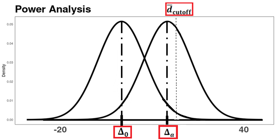
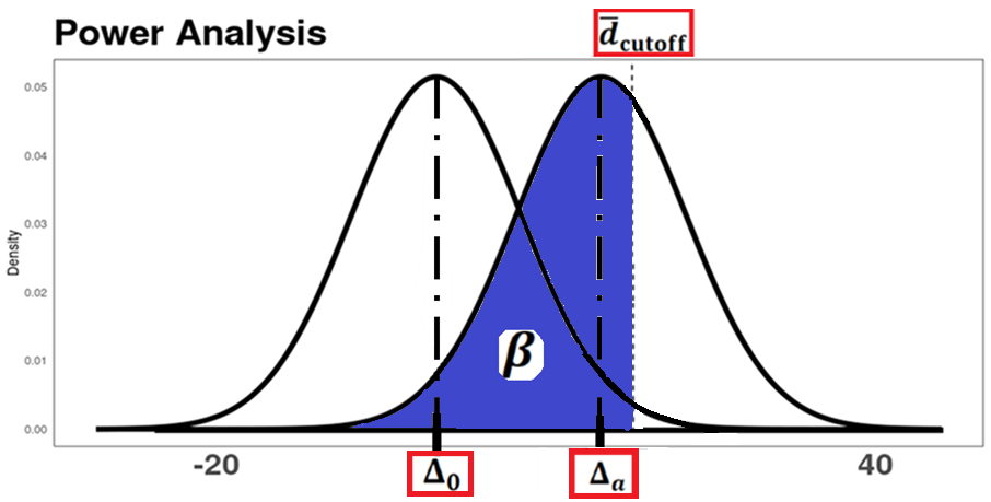
In the power graph below, clearly label and shade in the region on the graph that signifies the Type II error \(\beta\). Additionally, provide the values of \(\Delta_0\) and \(\Delta_a\), representing the mean difference under the null hypothesis and the meaningful difference for the alternative hypothesis, respectively.

Solution

i. \(\Delta_0 = 0\)

ii. \(\Delta_a = 15\)

The Type II error \(\beta\) is the probability of failing to reject \(H_0\) when \(H_a\) is true (i.e., when the true mean difference is \(\Delta_a = 15\)). On the power graph, this corresponds to the region under the alternative distribution (centered at \(\Delta_a = 15\)) that lies to the left of the cutoff value \(\bar{d}_\text{cutoff}\).

• \(\Delta_0 = 0\) is the mean under \(H_0\) (no difference between first and second child waiting times).

• \(\Delta_a = 15\) seconds is the meaningful difference specified as the alternative value for the power calculation.

Question 3e (8 pts)

Select the appropriate critical value for determining the cutoff value and calculate the cutoff value \(\bar{d}_\text{cutoff}\). Your answer must indicate both the critical value and the cutoff value.

qnorm(0.01, lower = FALSE)
[1] 2.326348

qnorm(0.025, lower = FALSE)
[1] 1.959964

qnorm(0.05, lower = FALSE)
[1] 1.644854

qnorm(0.95, lower = FALSE)
[1] -1.644854

Solution

Critical value: qnorm(0.05, lower = FALSE)

\[z = 1.644854\]

This is the upper \(\alpha = 0.05\) critical value, appropriate for the right-tailed test at significance level \(\alpha = 0.05\). (Note: since \(\sigma_D = 37\) is assumed known from prior research, a \(z\)-based cutoff is used.)

Cutoff value:

\[\bar{d}_\text{cutoff} = \Delta_0 + z \cdot \frac{\sigma_D}{\sqrt{n}} = 0 + 1.644854 \times \frac{37}{\sqrt{15}} = 1.644854 \times 9.5534 = \boxed{15.7139 \text{ seconds}}\]

Question 3f (7 pts)

Utilize the cutoff value calculated in part (e) to calculate the power of the test. Clearly set up the probability to be calculated and show the mathematical steps required to obtain the power of the test and select the correct code and output for computing the power of this test from the table below.

pnorm(1.239448,  lower.tail = FALSE)   # [1] 0.1075898
pnorm(1.239448,  lower.tail = TRUE)    # [1] 0.8924102
pnorm(0.07472524, lower.tail = FALSE)  # [1] 0.4702167
pnorm(0.07472524, lower.tail = TRUE)   # [1] 0.5297833
pnorm(0.3898356, lower.tail = FALSE)   # [1] 0.3483291
pnorm(0.3898356, lower.tail = TRUE)    # [1] 0.6516709

Solution

Power is the probability of correctly rejecting \(H_0\) when the true mean difference is \(\Delta_a = 15\):

\[\text{Power} = P\!\left(\bar{D} > \bar{d}_\text{cutoff} \mid \Delta = \Delta_a\right) = P\!\left(Z > \frac{\bar{d}_\text{cutoff} - \Delta_a}{\sigma_D / \sqrt{n}}\right)\]

Substituting:

\[= P\!\left(Z > \frac{15.71388 - 15}{37/\sqrt{15}}\right) = P(Z > 0.07472524)\]

Correct R code and output:

pnorm(0.07472524, lower.tail = FALSE)
[1] 0.4702167

\[\boxed{\text{Power} = 0.4702}\]

The test has only about 47% power to detect a true mean difference of 15 seconds with \(n = 15\) households at \(\alpha = 0.05\). This relatively low power reflects the small sample size relative to the variability (\(\sigma_D = 37\) seconds).

---

Problem 4 (20 points) — Sampling Distribution of Undergraduate Weights

Problem 4 Setup

Suppose weights of undergraduate students from Lumia University come from a minor positively skewed population with an average weight of 180 lb and with a standard deviation of 20 lb. A researcher randomly selects a sample of 40 undergraduate students from this population.

Question 4a (4 pts)

What is the distribution of the mean weights of the 40 undergraduate students? Clearly specify the name of the distribution and its parameters.

Solution

By the Central Limit Theorem, since \(n = 40 \geq 30\), the sampling distribution of \(\bar{X}\) is approximately normal regardless of the population’s positive skew:

\[\bar{X} \sim \text{Normal}\!\left(\mu_{\bar{X}} = 180,\ \sigma_{\bar{X}} = \frac{20}{\sqrt{40}}\right)\]

where

\[\sigma_{\bar{X}} = \frac{20}{\sqrt{40}} = \sqrt{10} \approx 3.1623 \text{ lb} \qquad \left(\sigma_{\bar{X}}^2 = 10\right)\]

Question 4b (8 pts)

What is the probability of the mean weight of the 40 undergraduate students being less than 175 lb? Clearly set up the probability to be calculated and show the mathematical steps required to obtain the probability. You may use the following R output in your calculations.

pnorm(-0.25, lower.tail = TRUE)    # 0.4012937
pnorm(-0.25, lower.tail = FALSE)   # 0.5987063
pnorm(-1.58, lower.tail = TRUE)    # 0.05705343
pnorm(-1.58, lower.tail = FALSE)   # 0.9429466
pnorm(-2.53, lower.tail = TRUE)    # 0.005703126
pnorm(-2.53, lower.tail = FALSE)   # 0.9942969

Solution

\[P(\bar{X} < 175) = P\!\left(Z < \frac{175 - 180}{20/\sqrt{40}}\right) = P\!\left(Z < \frac{-5}{3.1623}\right) = P(Z < -1.58)\]

From R output:

pnorm(-1.58, lower.tail = TRUE)
# 0.05705343

\[\boxed{P(\bar{X} < 175) = 0.0571}\]

Question 4c (8 pts)

What is the 99th percentile of the mean weight of the 40 undergraduate students? You may use the following R output in your calculations. Show your work.

qnorm(0.01/2, lower.tail = FALSE)   # 2.575829
qnorm(0.01,   lower.tail = FALSE)   # 2.326348
qnorm(0.04/2, lower.tail = FALSE)   # 2.053749
qnorm(0.04,   lower.tail = FALSE)   # 1.750686

Solution

The 99th percentile satisfies \(P(\bar{X} < \bar{x}_{0.99}) = 0.99\), which means \(P(Z > z) = 0.01\).

From R output: qnorm(0.01, lower.tail = FALSE) gives \(z = 2.326348\).

\[\bar{x}_{0.99} = \mu_{\bar{X}} + z \cdot \sigma_{\bar{X}} = 180 + 2.326348 \times \frac{20}{\sqrt{40}} = 180 + 2.326348 \times 3.1623 = \boxed{187.3566 \text{ lb}}\]

---

Problem 5 (32 points) — Pharmaceutical Regulation Hypothesis Test

Problem 5 Setup

For all pharmaceutical companies producing pills of Medicine A, federal regulations mandate that the ratio of the average weight to a fixed field standard value must not exceed 1.2. For Medicine A, this fixed field standard is 210 mg.

Question 5a (4 pts)

Formulate the government regulation requirement as an inequality using the average weight (\(\mu\)) of the pills. The inequality should be structured to place the average weight of the pills on one side by itself and a numerical value on the other side. How does this value relate to the hypothesis we formulate regarding the average weight of the pills?

Solution

Starting from the regulatory requirement:

\[\frac{\mu}{210} \leq 1.2 \implies \mu \leq 252\]

The value 252 mg is the null value for the hypothesis test. It represents the maximum allowable average pill weight under the regulation; any average exceeding 252 mg indicates non-compliance.

Question 5b (4 pts)

Placebo-Potion Pharmaceuticals was selected during the initial screening to conduct a formal hypothesis test, with \(n = 150\), \(\alpha = 0.01\), on whether the average pill weight exceeds the regulatory limit, indicating failure to meet the regulation. State the appropriate null and alternative hypotheses.

Solution

Step 1 — Parameter of interest: Let \(\mu\) represent the true mean weight (in mg) of Medicine A pills produced by Placebo-Potion Pharmaceuticals.

Step 2 — Hypotheses:

\[H_0: \mu \leq 252 \quad \text{(company meets regulation)}\]

\[H_a: \mu > 252 \quad \text{(company fails to meet regulation)}\]

This is a right-tailed test because the regulatory violation occurs when \(\mu\) exceeds 252 mg.

Question 5c (16 pts)

Placebo-Potion Pharmaceuticals collected an SRS from their production lines accordingly, and found that the sample mean was 256.5 mg and the sample standard deviation was 25 mg.

Part i (6 pts): Compute the appropriate test statistic. Show all work.

Part ii (3 pts): Select the appropriate code to compute the \(p\)-value from the table below.

# (A) pnorm(test_statistic)
# (B) pt(test_statistic, df = 150)
# (C) pt(test_statistic, df = 149)
# (D) pnorm(test_statistic, lower.tail = FALSE)
# (E) pt(test_statistic, df = 150, lower.tail = FALSE)
# (F) pt(test_statistic, df = 149, lower.tail = FALSE)
# (G) pnorm(abs(test_statistic), lower.tail = FALSE)
# (H) pt(abs(test_statistic), df = 150, lower.tail = FALSE)
# (I) pt(abs(test_statistic), df = 149, lower.tail = FALSE)

Part iii (9 pts): The \(p\)-value was found to be 0.0145 using the appropriate test statistic and code from above. State the decision and provide a formal conclusion about Placebo-Potion Pharmaceuticals’ compliance with the regulation based on this hypothesis test.

Solution

Part i — Test statistic:

Since \(\sigma\) is unknown, we use a one-sample t-test. With \(\bar{x} = 256.5\), \(\mu_0 = 252\), \(s = 25\), \(n = 150\):

\[t_\text{TS} = \frac{\bar{x} - \mu_0}{s/\sqrt{n}} = \frac{256.5 - 252}{25/\sqrt{150}} = \frac{4.5}{2.0412} = \boxed{2.2045}\]

Degrees of freedom: \(df = n - 1 = 149\).

Part ii — p-value code:

Answer: (F) pt(test_statistic, df = 149, lower.tail = FALSE)

This is a right-tailed test (\(H_a: \mu > 252\)), so the \(p\)-value is the upper-tail probability. We use lower.tail = FALSE with \(df = n - 1 = 149\) (not 150).

Part iii — Decision and conclusion:

Step 3 — Test statistic and p-value: \(t_\text{TS} = 2.2045\), \(df = 149\), \(p\text{-value} = 0.0145\).

Step 4 — Conclusion: Since the \(p\)-value \(= 0.0145 > \alpha = 0.01\), we fail to reject \(H_0\).

At the \(\alpha = 0.01\) significance level, the data do not provide sufficient evidence to conclude that the average weight of Medicine A pills at Placebo-Potion Pharmaceuticals exceeds the regulatory limit of 252 mg. In other words, it appears the company meets the regulation requirements.

Question 5d (6 pts)

In addition to the hypothesis test, the company was instructed to establish a confidence region for the true mean weight of the pills. Based on the results of the hypothesis test, which confidence region selection aligns most closely with those findings?

Part i (3 pts) — Type:

1. Confidence interval

2. Lower confidence bound

3. Upper confidence bound

Part ii (3 pts) — Interval/Bound Values:

1. (251.17, 261.83)

2. (253.17, 259.83)

3. \((251.6997,\ \infty)\)

4. \((253.6997,\ \infty)\)

5. \((-\infty,\ 261.3003)\)

Solution

Part i — Answer: (C) Upper confidence bound

Because the regulatory concern is with the upper end of \(\mu\) — the question is whether \(\mu\) might be too high — an upper confidence bound is the appropriate confidence region. It provides the highest plausible value for \(\mu\) and aligns with the right-tailed hypothesis test structure.

Part ii — Answer: (E) \((-\infty,\ 261.3003)\)

The 99% upper confidence bound is:

\[\text{UCB} = \bar{x} + t_{0.01,\,149} \cdot \frac{s}{\sqrt{n}} = 256.5 + 2.3517 \times \frac{25}{\sqrt{150}} = 256.5 + 4.8003 = 261.3003\]

where \(t_{0.01,\,149} \approx 2.3517\) (from R: qt(0.01, df=149, lower.tail=FALSE)).

The 99% upper confidence bound is \((-\infty,\ 261.3003)\). Since this bound contains \(\mu_0 = 252\), it is consistent with failing to reject \(H_0: \mu \leq 252\) at \(\alpha = 0.01\).